 Andrey V. Podlazov
PhD in Physics and Mathematics, senior researcher at RAS Keldysh Institute of Applied Mathematics, [email protected]
Spatio-temporal Decomposition of Vote Returns: The Case of Moscow Elections in 2012–18
Abstract
A method is proposed for the spatio-temporal decomposition of the returns of several votes held in the same set of territories. For different types of turnout – pro-government turnout, opposition turnout and spoiled-ballot turnout – historical and geographical components are identified as the zeroth and first principal components of the singular value decomposition of the turnout matrices. A natural normalisation of the decomposition components is introduced, giving them a simple and transparent interpretation. The toolkit developed here is applied to a series of electoral events held in Moscow in 2012–18. These events are unique in modern Russia in that their vote returns were virtually unaffected by fraud. The article examines the relationships between the spatial components in the decomposition of different types of turnout and demonstrates the influence of voters' educational level on these components. It also provides a brief analysis of the temporal components of the decomposition in the context of the political changes taking place at the time.
Introduction
The development of electoral statistics as applied to Russian data has been focused primarily on detecting fraud in these data and reconstructing the true voting returns [1; 2; 3; 5; 6; 7; 8; 9; 14; 23; 24; 25; 26; 27; 28; 29; 30; 31; 32; 33; 34; 35; 36; 37; 38; 39]. For a researcher, however, using a measuring instrument takes precedence over repairing and calibrating it. Electoral events are, in effect, large-scale social surveys that provide exceptionally rich material for sociopolitical research, which constitutes the second major area of electoral statistics [10; 11; 12; 13; 15; 16; 17; 18; 19; 20; 21; 22; 23; 40; 41]. Yet such studies are very often carried out without regard to the reliability of the available data, leaving open the question of the extent to which electoral fraud affects the results of the analysis.
After the mass protests of the winter of 2011–12, fraud in vote returns in Moscow took a sharp decline. For several years, this restored to voting its important function as a reliable source of sociological data for studying voters' political preferences and activity.
This article considers five electoral events held in Moscow in 2012–18 in which voters were offered a single list of alternatives. These were the votes in the presidential elections of 2012 and 2018, the Moscow mayoral elections of 2013 and 2018, and the 2016 election of State Duma deputies by party lists. The returns of these votes were almost unaffected by fraud [30], which, regrettably, gradually re-emerged later.
Sequential monitoring of the same territories not only places the phenomenon under study in its spatio-temporal dimension, but also potentially makes it possible to separate its spatial and temporal components, which is what will be done below. The present study is methodological rather than political-science-oriented. Its main focus is on how to process data. At the same time, it was of course impossible to refrain from examining what exactly was happening, where and when.
The analysis uses official vote returns published by the Moscow City Election Commission (http://www.moscow-city.izbirkom.ru), with detail down to individual polling stations. The unit of analysis is the region, which in most cases is identical to the municipal district. For the city within its administrative boundaries before 1 July 2012, the polling stations located in each municipal district always fall under the corresponding territorial election commission. After that date, Moscow’s boundaries were substantially expanded through the incorporation of a number of districts of Moscow Oblast, which slightly enlarged two districts of the Western Administrative Okrug (Skolkovo, as a detached area, was incorporated into Mozhaisky District, while the detached areas of Konezavod, VTB and Rublyovo-Arkhangelskoye were incorporated into Kuntsevo District) and also created the Troitsky and Novomoskovsky Administrative Okrugs (TAO and NAO). Since the municipal districts of the TAO and NAO are sparsely populated, this study instead uses synthetic regions defined by the areas covered by the Troitskaya (the settlements of Voronovskoye, Kievsky, Klyonovskoye, Krasnopakhorskoye, Mikhailovo-Yartsevskoye, Novofyodorovskoye, Pervomayskoye, Rogovskoye and Shchapovskoye, as well as the Troitsk urban okrug), Sosenskaya (the settlements of Voskresenskoye, Mosrentgen, Sosenskoye and Ryazanovskoye, as well as the Shcherbinka urban okrug) and Novomoskovskaya (the settlements of Vnukovskoye, Desyonovskoye, Kokoshkino, Marushkinskoye, Moskovsky and Filimonkovskoye) territorial election commissions in 2018 (on the maps presented below, the boundaries of the New Moscow districts are shown as of that date, without taking into account the administrative changes that occurred in 2024). The names of these regions are the same. For 2013 and 2016, the NAO was manually divided into regions according to the location of polling stations. For 2012, New Moscow polling stations are not considered, since at that time they still belonged to Moscow Oblast, where the reliability of vote returns is highly questionable. Thus, the dataset contains data for 125 regions for 2012 and for 128 regions for 2013–18.
Only vote returns from voters' place of residence are considered. Special polling stations, where voting takes place at a temporary place of stay (pre-trial detention centres, hospitals, care homes, military units, continuous-flow manufacturing facilities, ships, railway stations and similar locations) are excluded, since the voters assigned to them are restricted both in their access to information about candidates or parties and in their freedom to decide whether to take part in the vote. Moreover, for many such polling stations, voter lists are compiled on the basis of actual turnout, which makes turnout a fictitious quantity. Polling stations are identified as special by their numbers (3200 and above in 2012, and 3600 and above from 2013 onwards). Overseas polling stations formally assigned to the city are not considered either.
For each electoral event and each polling station considered, the following quantities are calculated as shares of the registered electorate:
– pro-government turnout – the share of voters who supported the candidate or party of power;
– opposition turnout – the share of voters who supported other candidates or parties;
– spoiled-ballot turnout – the share of voters who spoiled their ballots.
There is little point in analysing the electoral performance of individual opposition candidates or parties separately, since both their political affiliation and the list of such candidates or parties vary substantially from one electoral event to another. Moreover, in Russia the main distinction between the authorities and the opposition lies not so much in political orientation as in access to administrative resources; this is the rationale behind the simplified classification used here.
Treating spoiled ballots as a separate electoral choice (a form of protest voting) is justified by the absence of an "against all" option on the ballot, as well as by the exclusion from the analysis of polling stations at temporary places of stay, where spoiled ballots are quite likely to result from voters' physical limitations or from the semi-coercive nature of voting [29]. When voting takes place at the voter's place of residence, by contrast, it can be assumed that a voter who spoiled the ballot most likely came to the polling station precisely in order to do so.
Method of Analysis
Description of the Algorithm
The electoral events considered are denoted by the index \(e\), while the regions in which they were held are denoted by the index \(r\). For individual events, some regions may be missing, but the structure of the regions is treated as unchanged over the entire period under consideration. In all calculations, polling stations are assigned weights equal to the number of registered voters \(w_{er}\).
The first step in the analysis is to calculate, for each region, the median values of pro-government turnout, opposition turnout and spoiled-ballot turnout, \(t_{er}\) (the algorithm for calculating medians for weighted data can be found in the Appendix). Using median rather than mean turnout makes it possible to reduce the effects of sporadic fraud almost to zero and, to some extent, to compensate for the consequences of mobilising the voters vulnerable to administrative pressure (civil servants, members of the security agencies, employees of publicly funded institutions, social-sector workers, employees of state corporations, housing and utilities workers and similar categories of citizens). The point is that it is easiest to falsify returns at polling stations where support for the authorities is already high, while the activity of civil-society representatives capable of detecting and restraining fraud is, by contrast, low. At such polling stations, true pro-government turnout is already above the region median, so fraud no longer changes the value of the latter. Similarly, additional mobilisation of dependent voters inclined to support the authorities is most useful to the authorities precisely at those polling stations where such loyalist voters already make up a substantial share of the population, which in itself ensures high pro-government turnout. Finally, median filtering minimises distortions caused by the occasional inclusion in the analysed data of a small number of special polling stations, which sometimes have numbers from the general range.
For the median turnout of each type (pro-government, opposition or spoiled-ballot turnout) the following approximation is constructed:
\[t_{er}=k_ea_r+m_e+\epsilon_{er},\]
where the components \(m_e\) and \(k_e\) describe the political history, \(a_r\) describes the geography, and \(\epsilon_{er}\) is the residual. In other words, the task is to find the vectors of the zeroth component \(\begin{Vmatrix}m_e\end{Vmatrix}\), and of the first \(\begin{Vmatrix}a_r\end{Vmatrix}\) and \(\begin{Vmatrix}k_e\end{Vmatrix}\) components of the singular value decomposition of the turnout matrix \(\begin{Vmatrix}t_{er}\end{Vmatrix}\).
The condition of minimising the mean squared residual,
\[\sigma^2={\sum\nolimits_{e,r}{w_{er}\epsilon_{er}^2}}/{\sum\nolimits_{e,r}{w_{er}}}\rightarrow\min\]
gives the system of equations
\[\left\{\begin{matrix}m_e={\sum_r{w_{er}\left(t_{er}-k_ea_r\right)}}/{\sum_r{w_{er}}}\\k_e={\sum_r{w_{er}a_r\left(t_{er}-m_e\right)}}/{\sum_r{w_{er}a_r^2}}\\a_r={\sum_e{w_{er}k_e\left(t_{er}-m_e\right)}}/{\sum_e{w_{er}k_e^2}}\end{matrix}\right.,\]
which, when iterated alternately over the indices \(e\) and \(r\), makes it possible to obtain the decomposition of the turnout matrix. This iterative procedure quickly converges to stable values from any non-degenerate initial approximation, in which case a reasonable choice is \(m_e=0\), \(k_e=1\) and random \(a_r\).
Before the decomposition is performed, turnout values for each electoral event are normalised by dividing them by their standard deviations: \(t_{er}\rightarrow t_{er}/\sigma_e\), where
\[\frac{n_r(e)-1}{n_r(e)}\sigma_e^2=\frac{\sum_r{w_{er}t_{er}^2}}{\sum_r{w_{er}}}-\left(\frac{\sum_r{w_{er}t_{er}}}{\sum_r{w_{er}}}\right)^2,\]
and \(n_r(e)\) is the number of regions for which the returns of electoral event \(e\) are considered; this may be smaller than the total number of regions, \(n_r\), if there are gaps in the data. Normalisation equalises the influence of different events on the decomposition components and, after these components have been determined, is compensated for by multiplying the historical components back: \(m_e\rightarrow m_e\sigma_e\) и \(k_e\rightarrow k_e\sigma_e\).
Accuracy and Reliability of the Approximation Procedure
The decomposition described above approximates the pro-government, opposition and spoiled-ballot turnout values under consideration with errors of \(1.02\%\), \(0.71\%\) and \(0.095\%\) percentage points, respectively. In so doing, the decomposition explains more than \(99\%\) of the variance in turnout "for" and more than \(87\%\) of the variance in turnout "against." However, one should not be misled by the high level of determination, since it is achieved primarily because turnout values have a large variance, caused by differences in voter activity across electoral events. The purpose of the decomposition is not so much to obtain a highly accurate approximation of all elements of the turnout matrix as to eliminate the fluctuations affecting each individual matrix element by simplifying the description, that is, by reducing its dimensionality.
If we turn to the second principal component of the decomposition, that is, if we represent the residuals obtained earlier as
\[\epsilon_{er}=\tilde{k}_e\tilde{a}_r+\tilde{\epsilon}_{er}\]
and apply the toolkit described above to the variables with tildes (fixing \(\tilde{m}_e=0\)), the approximation errors decrease only to \(0.79\%\), \(0.56\%\) and \(0.076\%\) percentage points, respectively, that is, by less than a quarter. Such a minor refinement of the description does not justify introducing additional parameters. Admittedly, these parameters may be of interest in their own right, but analysing them lies beyond the scope of the present work. One noteworthy feature, which requires separate analysis, is the correlation pattern of the component \(\tilde{k}_r^\mathrm{spoiled}\): it correlates positively with \(k_r^\mathrm{opposition}\), and negatively with \(k_r^\mathrm{government}\), with coefficients of \(0.55\) and \(-0.72\).
Finally, the question of whether the data used here are indeed free from fraud large enough to overcome median filtering deserves separate attention. It is difficult to give a formal answer based on rigorous statistical methods, since applying them would require knowing the distribution of residuals. This distribution, however, combines the natural fluctuations of the data with the errors of the decomposition in an unpredictable way. Nevertheless, a detailed analysis allowed the author to identify indications of possible fraud.
For all polling stations in the city considered here, let us compare the mean turnout of each type with the weighted median of its region medians. The former is almost always slightly higher than the latter, especially for pro-government turnout. In the 2016 legislative election, however, the difference is anomalous: the mean exceeds the median by \(1.12\%\) percentage points, or \(9.3\%\). This provides grounds for examining the returns of this electoral event more closely. As can be seen from Fig. 1, for some regions this event does indeed show an overstatement of the actual turnout values relative to what is predicted by the decomposition. However, since even for this event the number of such regions is relatively small and the overstatement is not very large, these anomalies should not have a substantial effect on the overall results of the analysis.
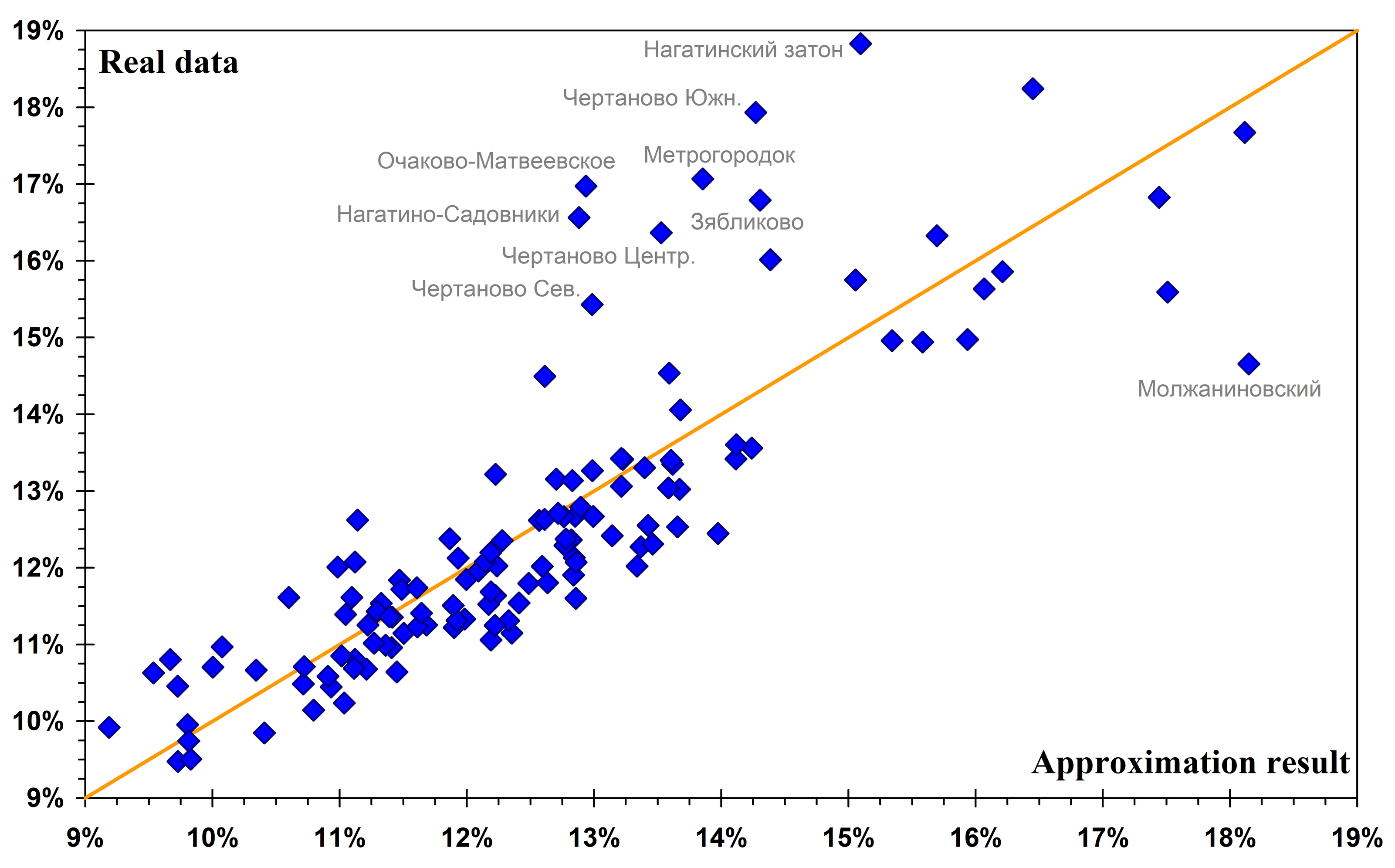
Fig. 1. Approximations of pro-government turnout in the 2016 legislative election. The diagonal corresponds to an exact approximation of the data, and the points cluster around it. However, eight regions deviate substantially from it in one direction, which may be the result of fraud. One regions deviates in the opposite direction; its indicators are subject to substantial fluctuations because it is very small – much smaller than the other city regions.
The author also considered electoral events held in Moscow in 2007–11 and in 2020. In these cases, however, fraud was large-scale, and it is unfortunately impossible to extend the approach described here to their returns. The share of regions where vote returns were substantially distorted by fraud is so large that all the statistical methods tested by the author treat the data from the few regions unaffected by fraud as outliers.
Moreover, not only objective methods but also human–machine methods of analysis prove useless in this case. Using the geographical component \(a_r\), determined from the returns of the 2012–18 electoral events, one may try to manually divide regions into suspicious and reliable ones for events outside this interval. This analysis is performed separately for each type of turnout, taking its specific features into account (fraud always increases pro-government turnout and decreases opposition turnout). In this case, reliable regions should lie on a straight line with slope \(k_e\) and intercept \(m_e\). However, there prove to be too few reliable regions and, more importantly, their sample is likely to be biased (as noted before, fraud occurs more often where voters are more loyal to the government). As a result, the historical components of the decomposition are determined with such large distortions that further analysis of them makes no sense.
Analysis of the Results
Normalisation
Since the decomposition components are determined only up to an arbitrary linear transformation, it is appropriate, before proceeding to further analysis, to normalise them in such a way that their values can be readily interpreted. The author is obliged to note that he is not aware of any studies in which this natural step is taken when principal component analysis is used. Normalisation is not necessary for presenting the results, but it greatly improves their clarity.
The following normalisation is used here: the values of political activity of the type under consideration, \(a=-{\scriptstyle\frac14}\) and \(a=+{\scriptstyle\frac14}\), should correspond to the upper and lower quartiles of the distribution of voters by that activity. To this end, the quartiles of the activity obtained from the decomposition, \(a({\scriptstyle\frac14})\) and \(a({\scriptstyle\frac34})\). The calculations use weights \(w_r=\sum_e{w_{er}}\) (the algorithm for calculating quantiles is described in the Appendix). Renormalisation is performed using the formulae \(a_r\rightarrow(a_r-\mu)/\gamma\), \(m_e\rightarrow m_e+\mu k_e\) and \(k_e\rightarrow\gamma k_e\), where \(\mu=\left(a({\scriptstyle\frac14})+a({\scriptstyle\frac34})\right)/2\) and \(\gamma=2\left(a({\scriptstyle\frac14})-a({\scriptstyle\frac34})\right)\). In addition, if the resulting values of \(k_e\) are negative (they all have the same sign), the final cosmetic adjustment is to change the signs of all \(k_e\) and \(a_r\) simultaneously.
As a result of this normalisation, one quarter of voters are characterised by activity below \(-{\scriptstyle\frac14}\), and one quarter by activity above \(+{\scriptstyle\frac14}\). The quantity \(k/2\) then acquires the meaning of the half-width of the distribution of voters by turnout of the type under consideration, so that \(k\) is hereafter referred to simply as the width of the distribution. If the distribution were uniform, this interpretation would be exact, but the real distribution is, of course, considerably wider. As can be seen from Fig. 2, the values \(a=-{\scriptstyle\frac12}\) and \(a=+{\scriptstyle\frac12}\) correspond approximately to the upper and lower deciles of the distribution; that is, when moving from the \(10\%\) least active voters to the \(10\%\) most active voters, their turnout of the type under consideration – in support of the authorities or the opposition, or through spoiled ballots – increases by approximately \(k\).
The value \(a=0\), as the arithmetic mean of the quartiles, approximately corresponds to the median of the distribution of voters by activity. Therefore, in what follows, \(m\) is treated as an estimate of the median of the distribution of voters by turnout of the type under consideration, without further reference to the approximate nature of this estimate. Fig. 2 shows that its deviations from the true median are small.
At the same time, the distribution of activities is asymmetric, since its tails are of different lengths. The tail for values \(a\gt 0\) is longer: in other words, there are regions with anomalously high activity of a given type, but no regions with anomalously low activity.
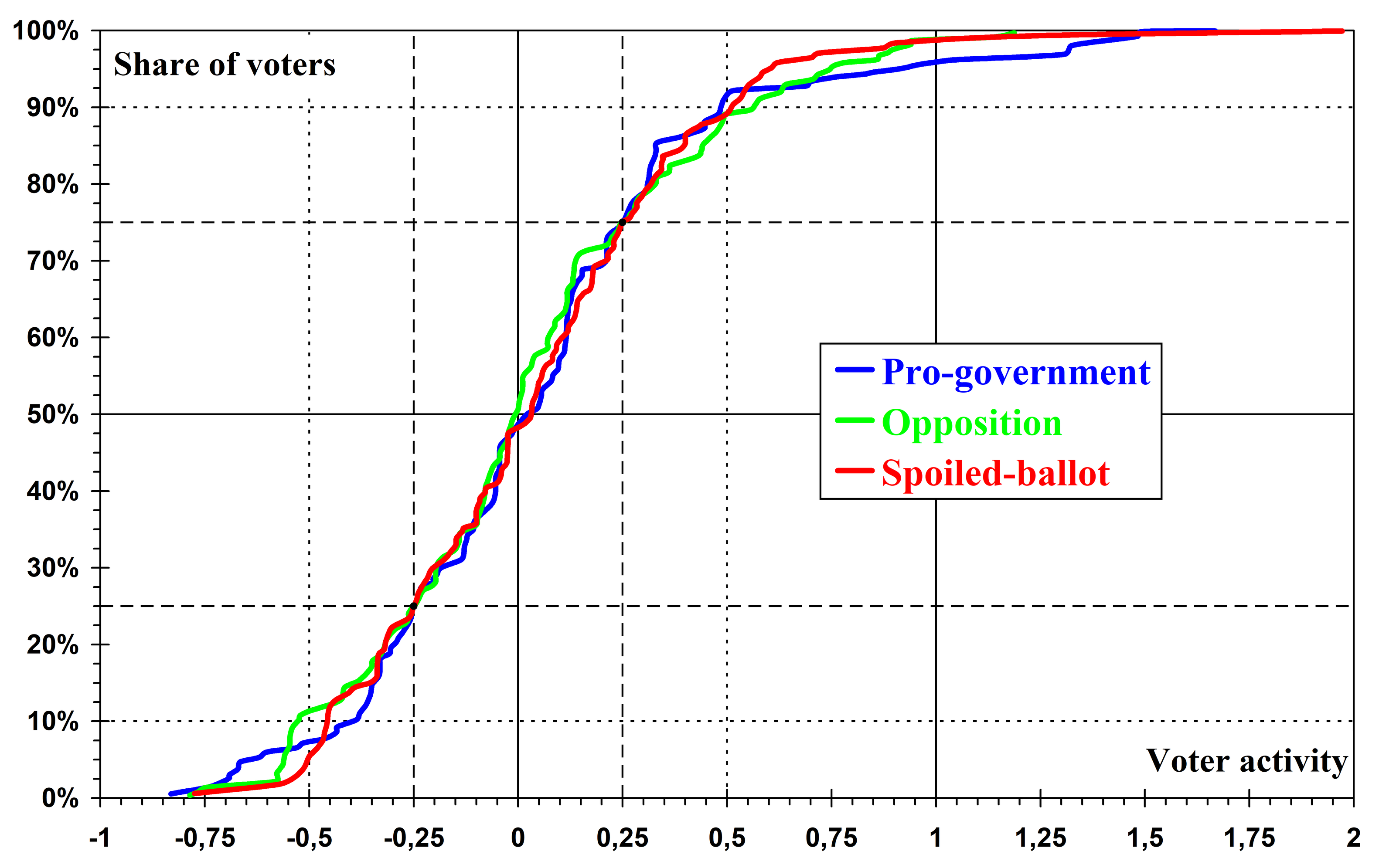
Fig. 2. Distribution of regions by voters' political activity. In these plots, regions are ordered by increasing abscissa, while the ordinate shows the cumulative share of voters living in them. The horizontal grid lines indicate the positions of the median (solid), the quartiles (dashed) and the deciles (dotted) of the distribution, while the vertical lines indicate the corresponding values of political activity – exact by definition for the quartiles and approximate for the deciles and the median. An additional solid vertical line at unit activity highlights the asymmetry of the distribution.
Political Geography
Fig. 3 presents maps of voters' political activity in Moscow. A region's location clearly has a substantial influence on the political preferences of its residents. Regions with high opposition activity tend to cluster towards the city centre, whereas regions with high pro-government activity are located closer to the city's historic boundaries or beyond them.
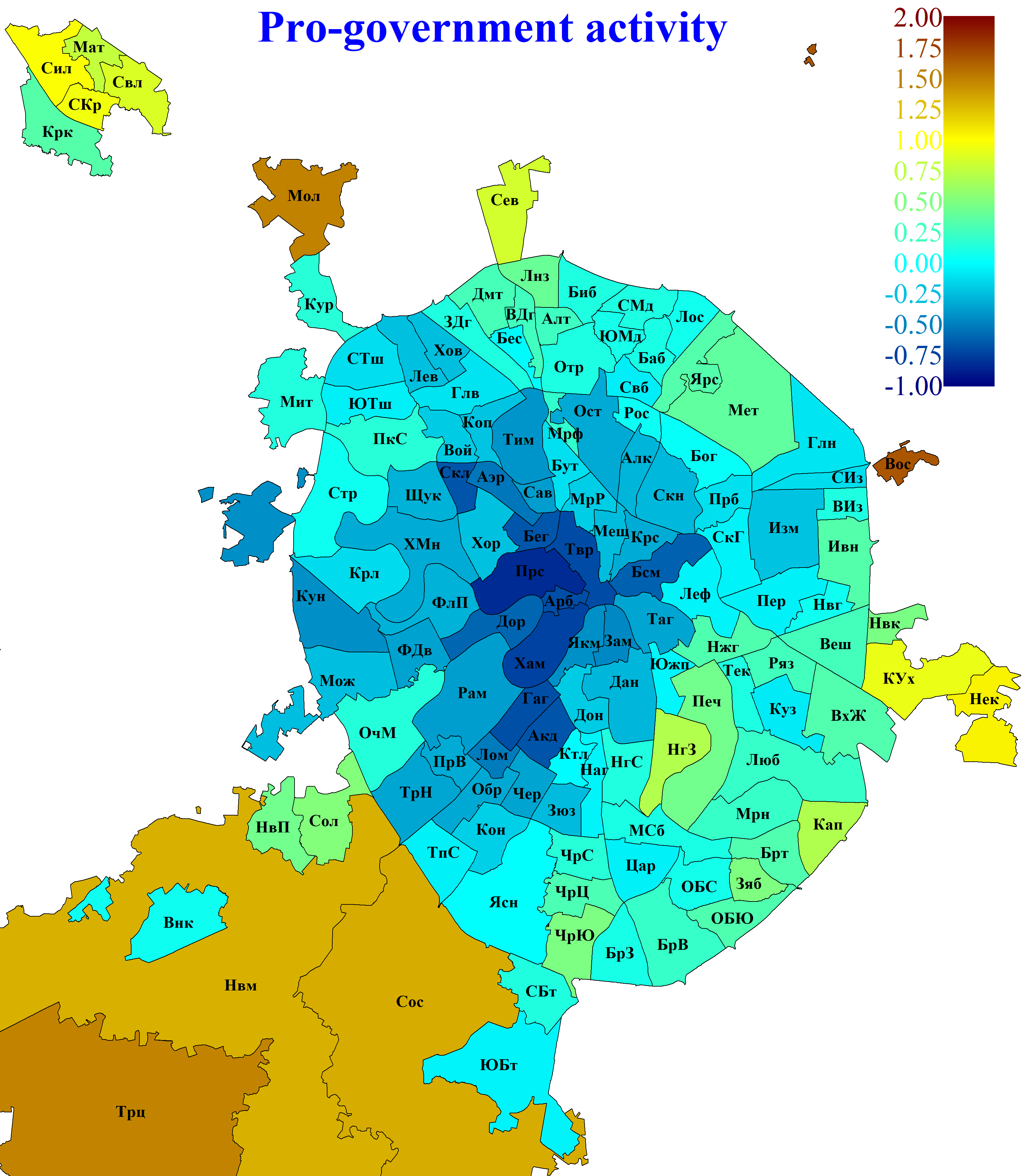
Fig. 3. Political activity of Moscow voters by region. A. Pro-government activity.
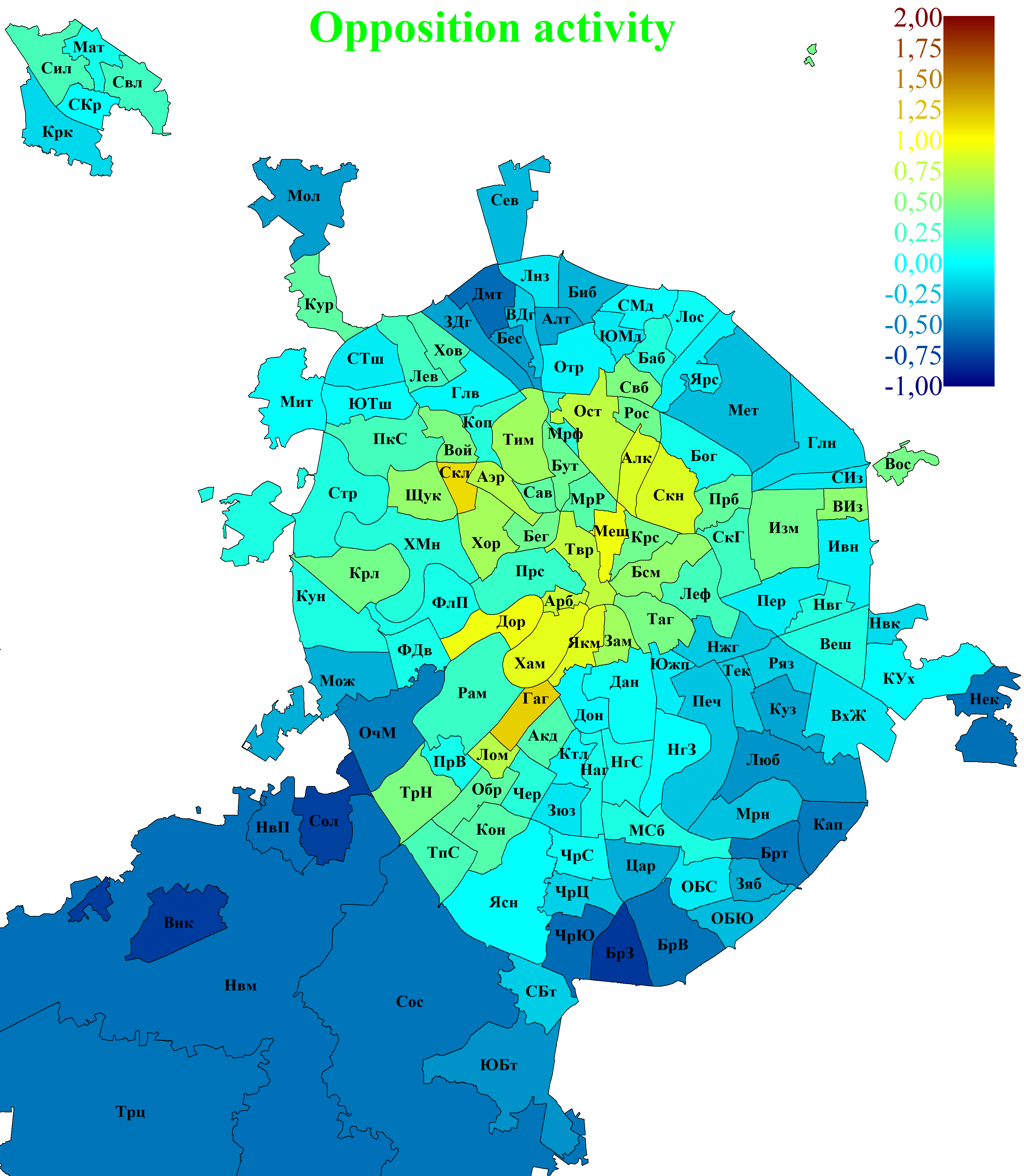
B. Oppositional activity.
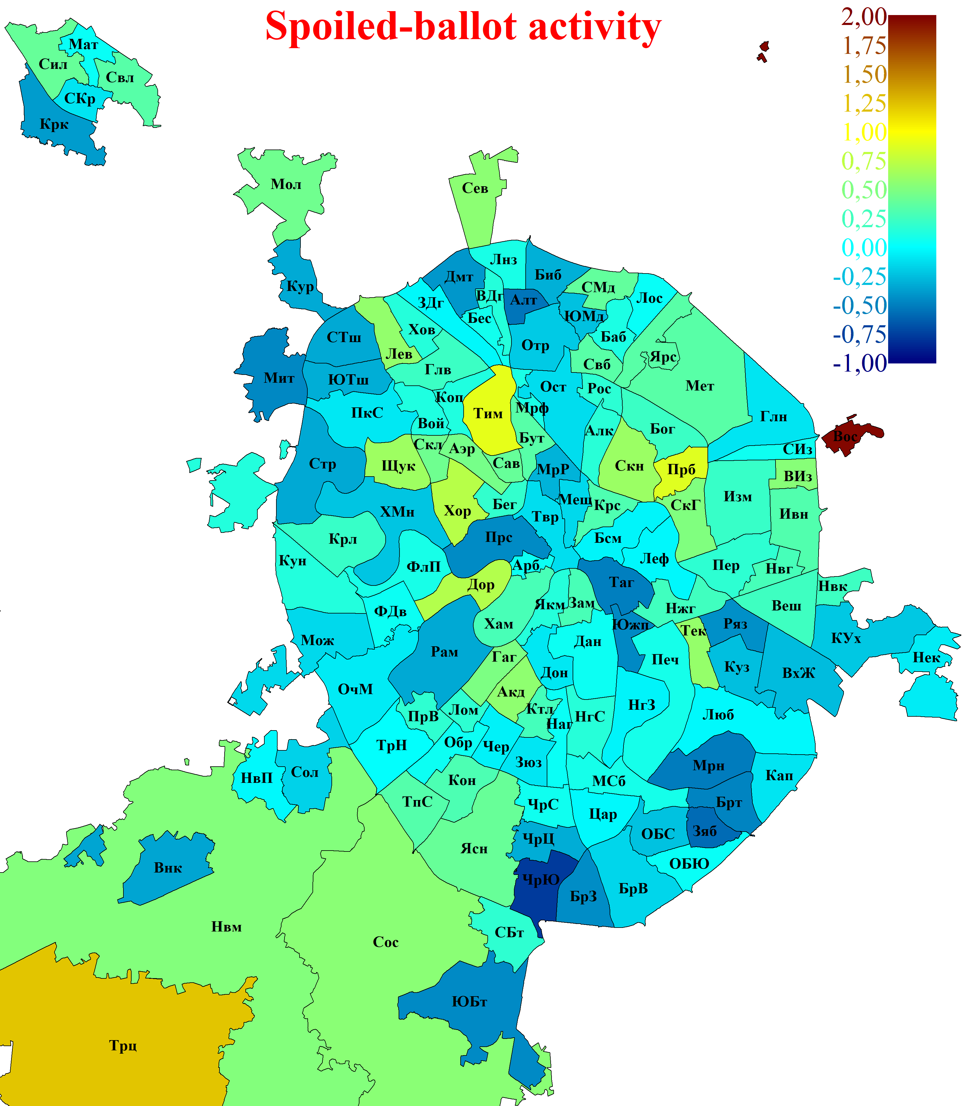
C. Ballot spoilage activity. The same colour scale is used for all three types of activity in order to make the data presentation comparable. Owing to the enormous size of the New Moscow regions, they are shown only in part, with the map cropped approximately along the south-western boundary of the Filimonkovskoye settlement.
Fig. 4 provides a direct comparison of the two main types of political activity. Their negative correlation is beyond doubt. It should be noted that this is not self-evident a priori, since an alternative hypothesis could have been formulated: that regions differ only in their overall level of political activity, which is divided more or less proportionally between the government and the opposition.
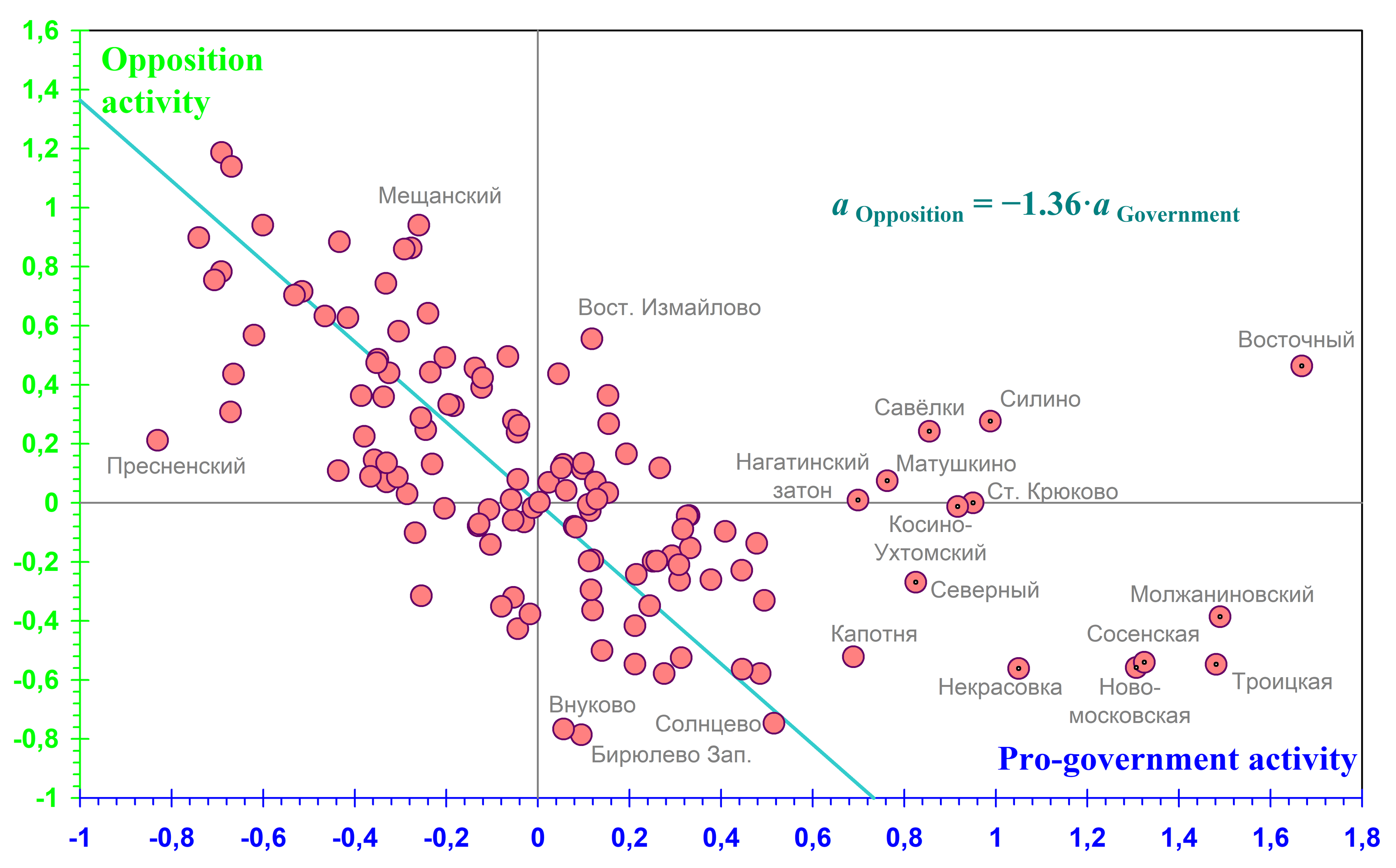
Fig. 4. Relationship between opposition and pro-government voter activity. For most regions, opposition activity is negatively correlated with pro-government activity. Data for 13 regions that do not lie on the line (shown with pin markers) were not used to determine its parameters.
It would be incorrect to establish the relationship between different types of activity using ordinary regression models, which assume that the explanatory variables are measured without error. However, since the activity measures are expressed in the same units and have similar ranges of variation, it is both permissible and appropriate to use a Deming regression model without an intercept. This model minimises the mean squared deviation of the points not along the response variable, but in the direction perpendicular to the regression line passing through the origin. When the regression parameters are estimated, regions are weighted by the number of voters averaged over all electoral events. In Fig. 4, the ratio of the scatter of points along the line to their scatter across it is \(2.57\), which is not very large, but still more than sufficient for the line to be identified reliably.
Among the regions that do not lie on the line, only Nagatinsky Zaton is located inside the MKAD (the Moscow Ring Road; from 1960 to 1984, it served as the city's administrative boundary); the remaining regions – Vostochny, Savyolki, Silino, Matushkino, Staroye Kryukovo, Kosino-Ukhtomsky, Severny, Molzhaninovsky, Nekrasovka, Sosenskaya, Troitskaya and Novomoskovskaya – lie outside it. Their residents show low opposition activity combined with anomalously high pro-government activity. This suggests that, in political terms, regions that geographically and/or historically belong rather to Moscow Oblast than to Moscow may differ substantially from the main body of metropolitan regions. The outlier status of Nagatinsky Zaton is most likely due to this region’s exceptional propensity for fraud.
As can be seen from Fig. 5, spoiled-ballot activity is positively correlated with opposition activity, which confirms the protest nature of spoiled ballots. At the same time, the linear relationship between these two types of activity is less pronounced than that between pro-government and opposition activity (see Fig. 4). Therefore, in Fig. 5, the ratio of the scatter of points along the line to their scatter across it is only \(1.63\). The regions of Vostochny and Troitskaya do not lie on the line. They are located outside the MKAD and display an intermediate, transitional type of behaviour, in which still-low opposition activity is combined with already-high spoiled-ballot activity.
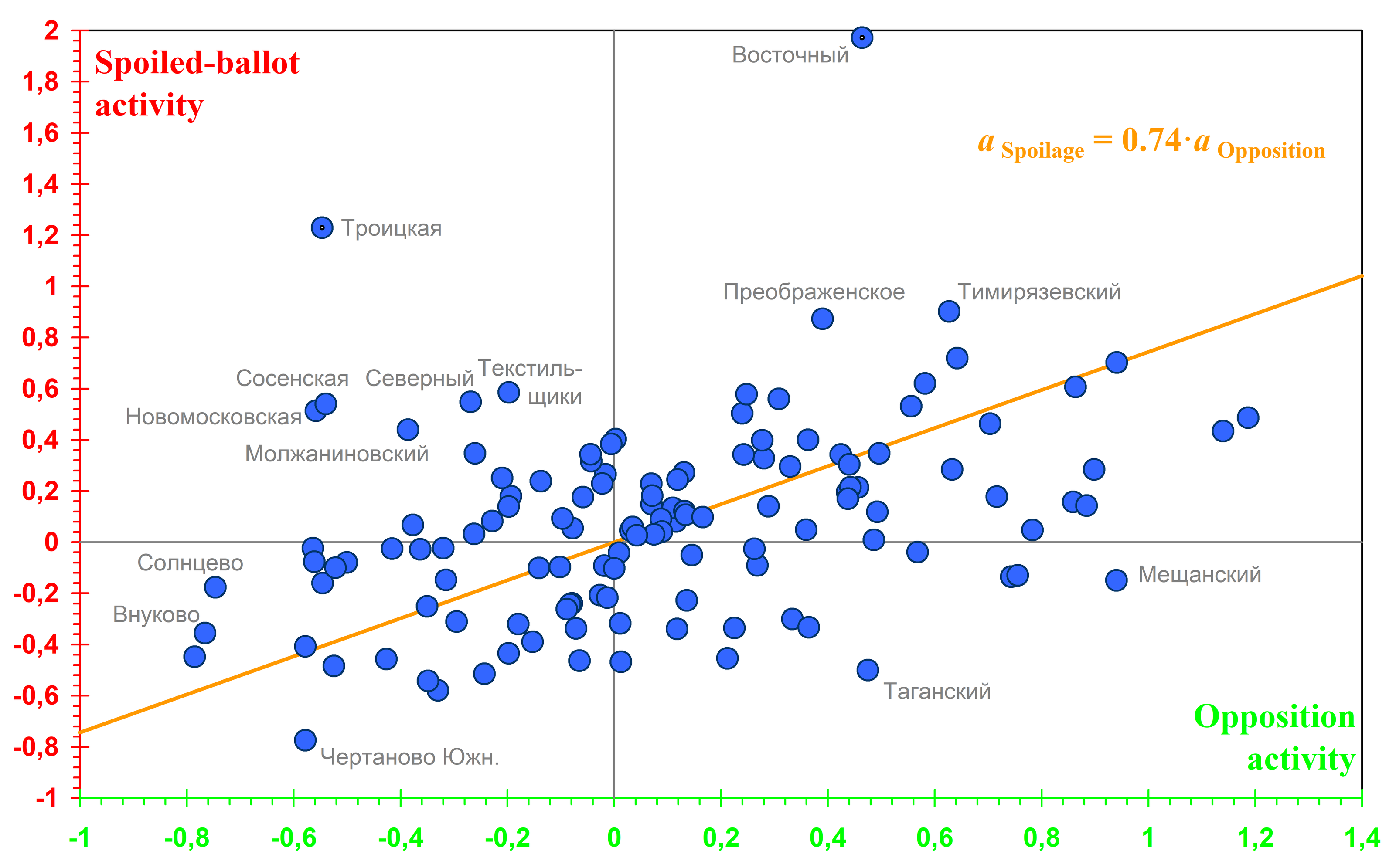
Fig. 5. Relationship between spoiled-ballot activity and opposition activity. For most regions, spoiled-ballot activity is positively correlated with opposition activity. Data for two regions that do not lie on the line (shown with pin markers) were not used to determine its parameters.
Determinants of Political Activity
As shown earlier in [29], the educational level of voters is an important determinant of election results in Moscow, enabling them to make independent decisions both about supporting particular political forces and about whether to take part in voting at all.
A more detailed analysis showed that what matters is not the educational level of the population as a whole, but that of its older segment, which is most dependent on the mass media. For younger voters, by contrast, additional sources of information (communication with colleagues and active use of the internet) appear to reduce the role played by educational differences (it is important to remember that the events in question took place roughly a decade ago, when mobile internet and social media were much less widespread than they are today). Therefore, the measure used here is the share of persons above working age who have completed higher education [4] (see Fig. 6).
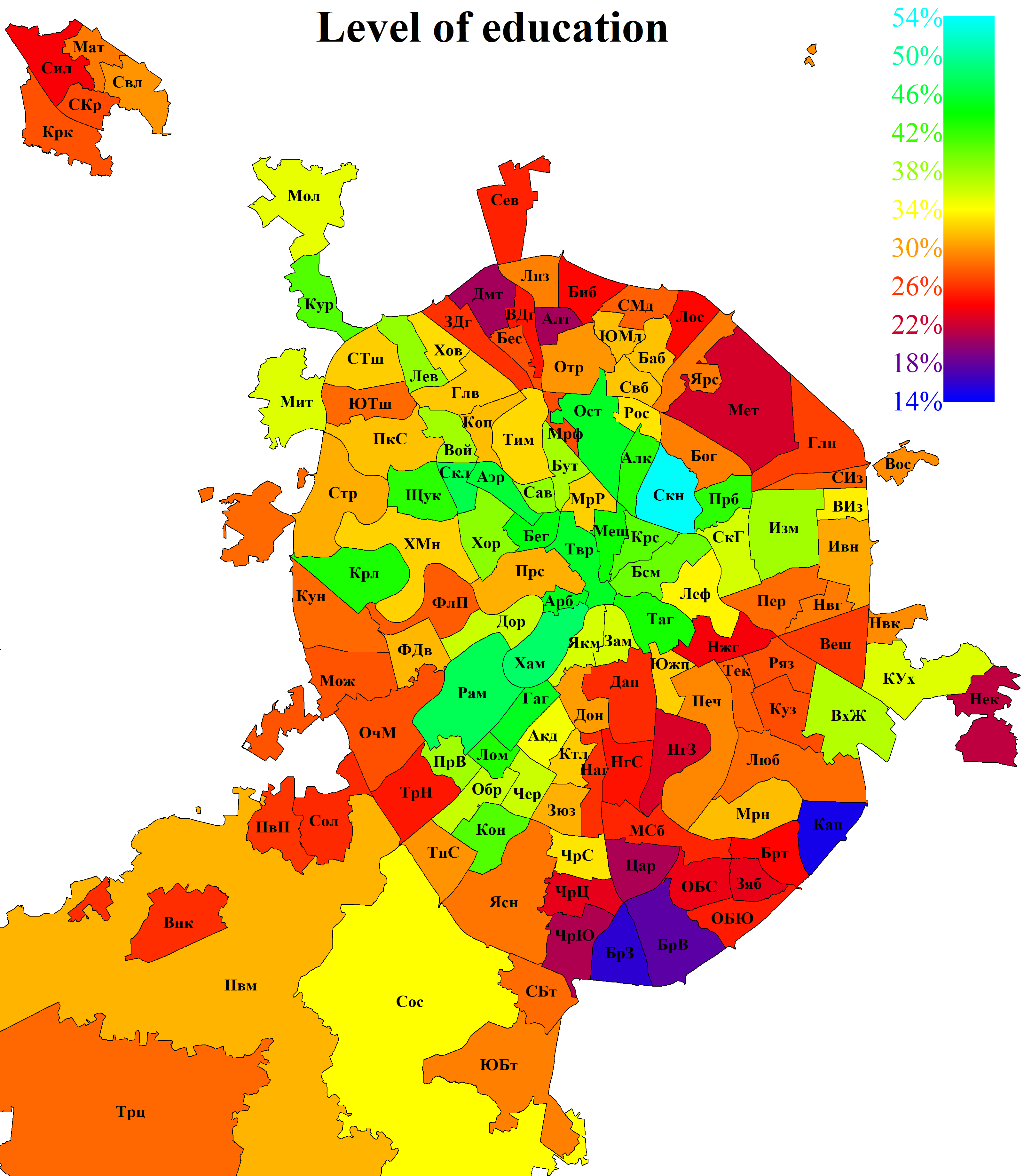
Fig. 6. Share of persons above working age with higher education. Based on data from the 2020 Russian Census. The share is measured relative to the number of persons who reported their educational level in the census questionnaire.
Figs. 7 and 8 show that the educational level of voters has a positive effect on opposition activity and a negative effect on pro-government activity. Importantly, there are no outlying points for opposition activity (Fig. 7), whereas such points are present for pro-government activity (Fig. 8). Therefore, the outlying points in Figs. 4 and 5 are caused specifically by the anomalous behaviour of provincial voters, who are sometimes prone to inflated support for the authorities (Fig. 4) and excessive number of spoiled ballots (Fig. 5).
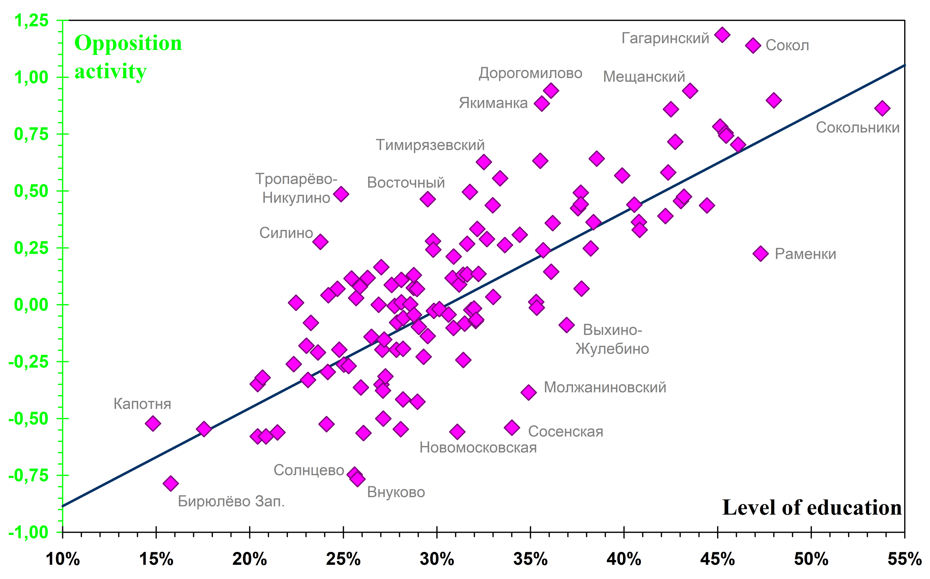
Fig. 7. Determination of opposition activity by educational level. The error of the linear approximation is 0.26 (biased estimate), and the correlation coefficient is 0.75. If the abscissa is taken to be the share of persons with higher education among those of voting age, rather than among those above working age, the error increases to 0.32, while the correlation coefficient decreases to 0.56.
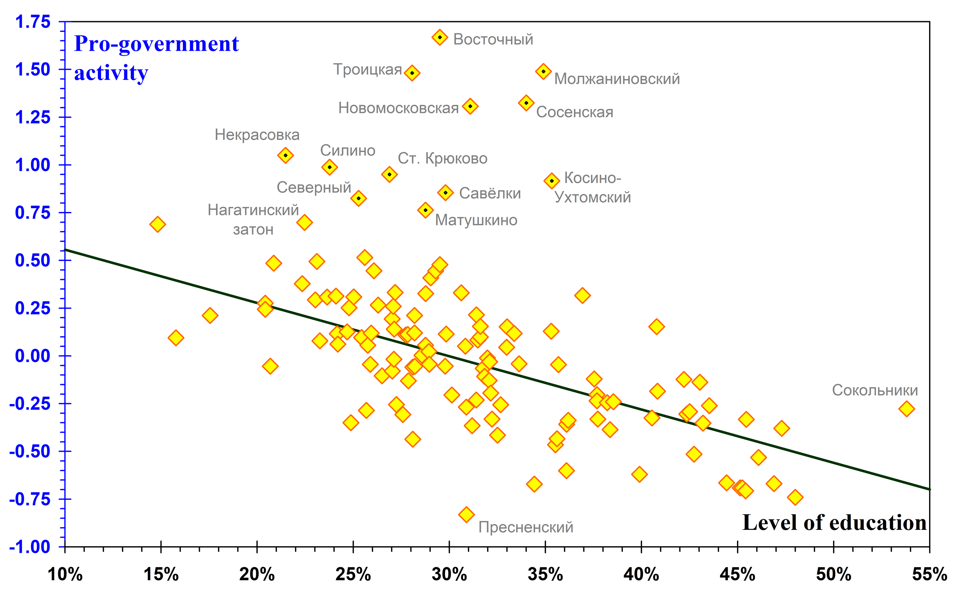
Fig. 8. Determination of pro-government activity by educational level. The figure is analogous to Fig. 7; here, however, 12 regions (shown with pin markers and the same as in Fig. 4, except for Nagatinsky Zaton) do not lie on the regression line. Their data were not used to determine its parameters. For the remaining regions, the error of the linear approximation is 0.25 (biased estimate), and the correlation coefficient is -0.70.
Political History
Fig. 9 shows changes in the component \(k_e\) over the electoral events considered for the different types of political activity. From a political-science perspective, the width of the distribution of voters by opposition turnout measures electoral competitiveness; the width of the distribution by pro-government turnout measures the authorities' ability to mobilise loyalist voters; and the width of the distribution by spoiled-ballot turnout measures the overall consequences of the use of administrative resources.
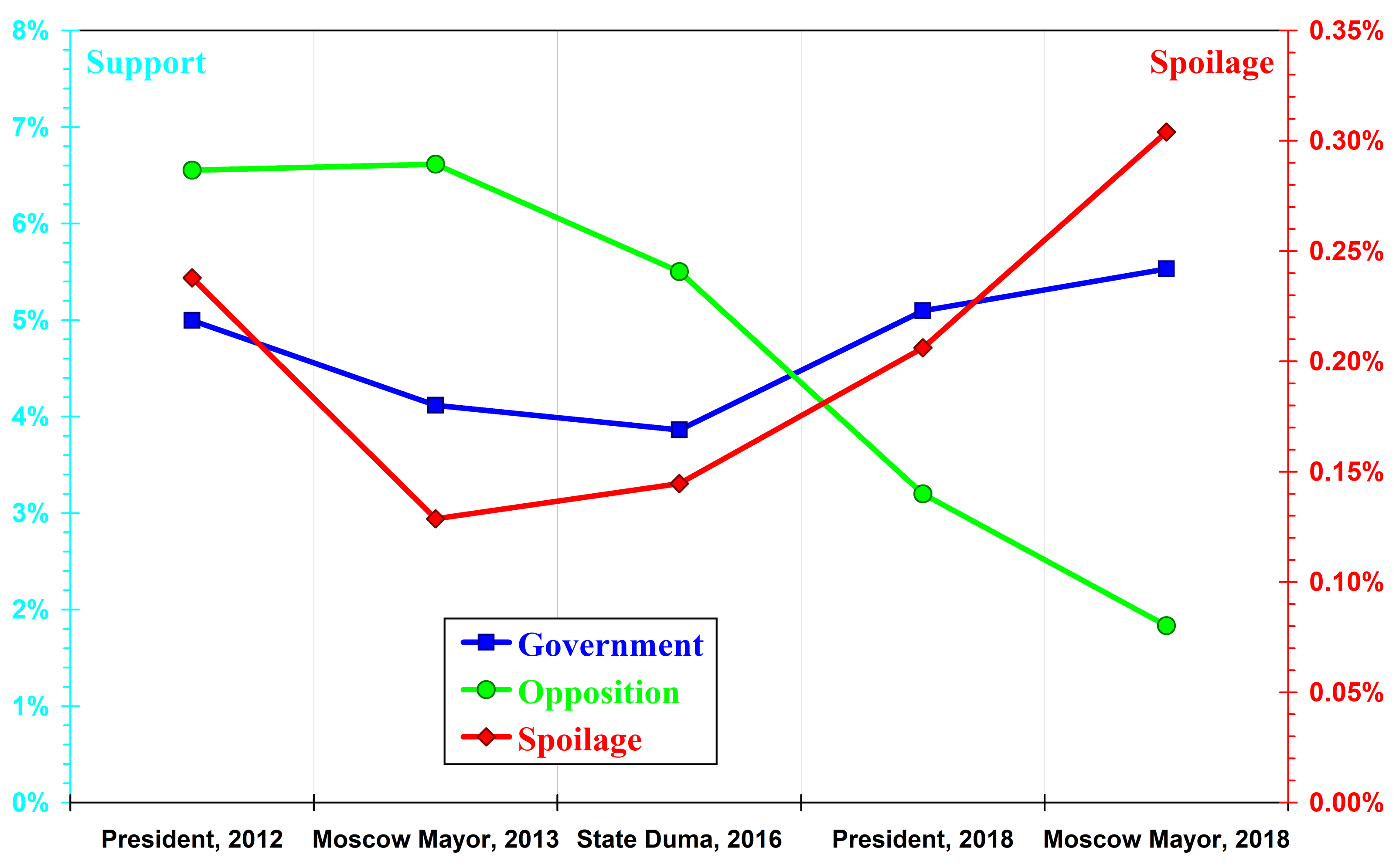
Fig. 9. Widths of the distribution of voters by turnout. This quantity characterises the dispersion of regions by turnout of the corresponding type. The left-hand axis shows the parameters for voting in support of the government and the opposition, while the right-hand axis shows those for protest voting.
The greater the number of different candidates or parties competing for election, the larger the share of voters in an opposition-leaning region who will find someone to vote for, thereby increasing the width of the distribution of voters by opposition turnout. Conversely, denying electoral participants registration or hindering their election campaigning means that some voters, finding no representatives of their interests, do not come to the polls at all. This brings opposition turnout in opposition-leaning and pro-government regions closer together, reducing the width of the distribution. This is exactly what the graph shows: electoral competitiveness was very high in 2012–13, began to decline in 2016 while still remaining high, and collapsed only in 2018. Here, however, the analysis concerns Moscow rather than Russia as a whole. In Moscow, the non-parliamentary Yabloko party came fourth, well ahead of the parliamentary A Just Russia, while parties that failed to cross the 5% threshold received, in total, more votes than the Communist party, which came second.
The government always limit its participation in elections to a single candidate or party. As a result, electoral events differ only slightly in the degree to which voters vulnerable to administrative pressure are mobilised, and the graph of the distribution width is almost horizontal.
The growing role of the government's administrative resources affects protest in two ways. On the one hand, the widening of the distribution of voters by spoiled-ballot turnout may result from declining electoral competitiveness, which leaves voters without options to support. On the other hand, dependent voters and members of their families who come to polling stations against their will sometimes spoil their ballots as a protest against the very fact of mobilisation. Taken together, these factors lead to an accelerating increase in the width of the distribution of protest turnout after 2013.
Fig. 10 shows changes in the component \(m_e\) over the electoral events considered for the different types of political activity. The median of the distribution of voters by turnout primarily reflects the type of electoral event. For mayoral elections, it is almost always lower than for presidential elections, the sole exception being spoiled-ballot turnout in the two 2018 elections. For parliamentary elections, this component behaves in a more complex way. In 2016, the median for the authorities was the lowest, while that for the opposition was among the highest. The reason for this divergence lies in the difference between elections to a single office and elections to a collective body. In the former, the winner takes all, so weaker candidates have reason to take part only in order to promote their ideas; in the latter, several parties can achieve success. This is why the medians for both opposition turnout and even spoiled-ballot turnout are relatively high in legislative election.
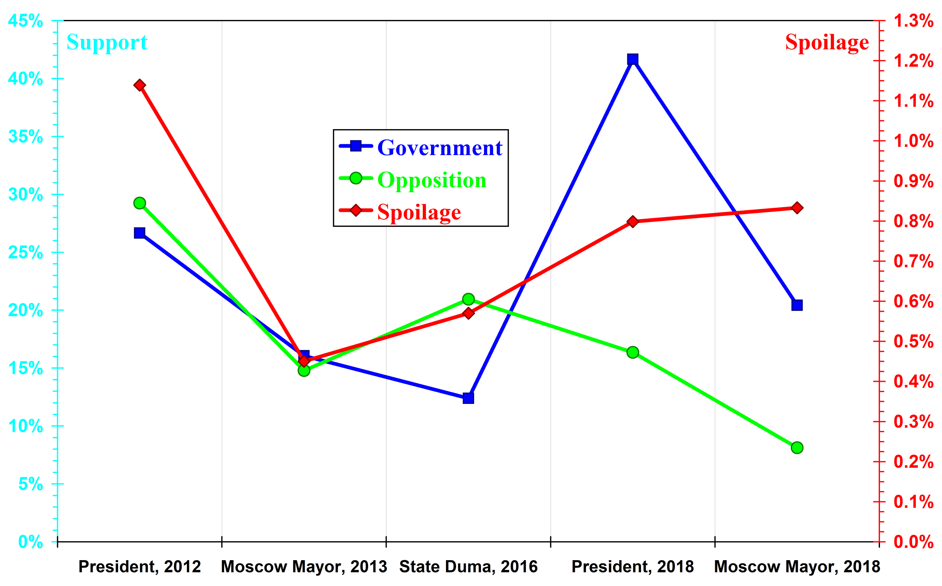
Fig. 10. Medians of the distribution of voters by turnout. This quantity gives the typical level of turnout of the corresponding type. The left-hand axis shows the parameters for voting in support of the government and the opposition, while the right-hand axis shows those for protest voting.
A comparison of the medians for the pairs of presidential elections (2012/18) and mayoral elections (2013/18) also reveals a decline in their competitiveness and an increase in the mobilisation of the loyalist electorate. For the opposition, which in 2018 was deprived of the opportunity to nominate its strongest candidates, the median is lower than in comparable elections in previous cycles, while for the authorities it is higher.
For spoiled-ballot turnout, the dynamics of the median of the voter distribution resemble the dynamics of its width, with the sole difference that in 2018 the growth of the median slowed and, unlike the width, it never exceeded the 2012 value. In other words, differences between regions in the level of protest sentiment are increasing faster than the overall level of such sentiment.
Conclusion
For electoral events with a single list of candidates or parties, and in the absence of large-scale fraud in vote returns, turnout of different types – pro-government turnout, opposition turnout and spoiled-ballot turnout – can be decomposed, with satisfactory accuracy, into geographical and historical components. The former characterises the political preferences and activity of voters in a given territory, while the latter characterise the parameters of the distribution of voters by turnout.
For Moscow elections in 2012–18, the dynamics of the historical component show a rapid and consistent decline in electoral competitiveness after 2013. This is associated with an increase in protest voting, for which both the overall level of spoiled-ballot turnout and, especially, its variation across regions are growing.
For most regions, the geographical component shows a negative correlation between pro-government and opposition activity, as well as a positive correlation between opposition and protest activity. The only exception is a subset of the most outlying regions, where no relationship between these types of activity is observed.
Electoral behaviour is largely determined by voters' educational level. The share of educated older residents determines opposition activity in all regions and pro-government activity in all regions except the most remote ones, which historically are closer to non-metropolitan than to metropolitan regions. This shows that the disruption of the relationship between these types of political activity in those areas is due to anomalously high support for the government there.
Appendix
Some statistical software packages that provide tools for calculating sample quantiles do so in a not entirely correct manner. Moreover, most packages do not allow sample values to be weighted. The corresponding algorithm is therefore given below.
Let there be a set of numbers \(x_i\), sorted in ascending order and taken with weights \(w_i\), \(i=1, 2, …n\), and suppose that it is necessary to determine \(x(q)\), the quantile at a given level \(q\).
Denote the sums of weights by \(s_i=\sum_{j=1}^i{w_j}\) and \(\bar{s_i}=s_n-s_i\). Each sample value \(x_i\) corresponds to its exact quantile level \(q_i=(s_i-w_i/2)/s_n\), while the approximate value of the required quantile is found by linear interpolation between the values \(x_i\) and \(x_{i+1}\), where the index \(i\) is such that \(q_i\leq q\leq q_{i+1}\). This condition can be rewritten as \(-w_{i+1}\leq r_i\leq w_i\), introducing the notation \(r_i=2(\bar{q}s_i-q\bar{s_i})\), where \(\bar{q}=1-q\). Then
\[x(q)=\frac{x_i(r_i+w_{i+1})-x_{i+1}(r_i-w_i)}{w_i+w_{i+1}}.\]
If \(q={\scriptstyle\frac12}\), that is, if the median is sought, then \(r_i=s_i-\bar{s_i}\), and the condition on the index \(i\) simplifies to \(d_i\leq 0\leq d_{i+1}\), where \(d_i=s_{i-1}-\bar{s_i}\). In this case,
\[\mathrm{med}x=\frac{x_id_{i+1}-x_{i+1}d_i}{w_i+w_{i+1}}.\]
Received 11.04.2026, revision received 01.05.2026.
References
- Buzin A.Yu., Grishin N.V., Kalinin K., Kogan D.L., Korgunyuk Yu.G., Mikhailov V.V., Ovchinnikov B.V., Shalaev N.E., Shen A., Shpilkin S.A., Shukshin I.A. Using Mathematical Methods for Electoral Fraud Detection. – Electoral Politics. 2020. No. 2 (4). P. 4. - http://electoralpolitics.org/en/articles/vozmozhnosti-matematicheskikh-metodov-po-vyiavleniiu-elektoralnykh-falsifikatsii
- Buzin A.Yu. Overview of Electoral Statistics for the 2025 Regional Head Elections. – Electoral Politics. 2025. No. 2 (14). P. 3. - https://electoralpolitics.org/en/articles/obzor-elektoralnoi-statistiki-vyborov-glav-regionov-v-2025-godu/
- Buzin A.Yu. The Modification of Sobyanin-Soukhovolsky Method. – Electoral Politics. 2019. No. 1. P. 2. - http://electoralpolitics.org/en/articles/modifikatsiia-metoda-sobianina-sukhovolskogo
- Itogi Vserossiyskoi perepisi naseleniya 2020 goda po g. Moskve [Results of the 2020 All-Russian Population Census for Moscow]. Vol. 3. Obrazovaniye [Education]. Table 1. Naseleniye po vozrastu, polu i urovnyu obrazovaniya po munitsipalnym obrazovaniyam [Population by Age, Sex and Level of Education by Municipal District]. URL: https://77.rosstat.gov.ru/storage/mediabank/том%203.%20Таблица%201.xlsx (accessed 26.05.2026). (In Russ.) - https://77.rosstat.gov.ru/storage/mediabank/том%203.%20Таблица%201.xlsx
- Kobak D., Shpilkin S., Pshenichnikov M.S. Integer percentages as electoral falsification fingerprints. – Ann. Appl. Stat. 2016. Vol. 10. No. 1. P. 54–73. DOI: 10.1214/16-AOAS904
- Kobak D., Shpilkin S., Pshenichnikov M.S. Putin’s peaks: Russian election data revisited. – Significance. 2018. Vol. 15. No. 3. P. 8–9. DOI: 10.1111/j.1740-9713.2018.01141.x
- Kobak D., Shpilkin S., Pshenichnikov M.S. Statistical anomalies in 2011–2012 Russian elections revealed by 2D correlation analysis. – arXiv, 17.05.2012. URL: https://arxiv.org/abs/1205.0741 (accessed 26.05.2026). - https://arxiv.org/abs/1205.0741
- Kobak D., Shpilkin S., Pshenichnikov M.S. Statistical fingerprints of electoral fraud? – Significance. 2016. Vol. 13. No. 4. P. 20–23. DOI: 10.1111/j.1740-9713.2016.00936.x
- Kobak D., Shpilkin S., Pshenichnikov M.S. Suspect peaks in Russia’s “referendum” results. – Significance. 2020. Vol. 17. No. 5. P. 8–9. DOI: 10.1111/1740-9713.01438
- Korgunyuk Yu.G. Electoral Cleavage Structure: 2021 State Duma Election. – Electoral Politics. 2023. No. 1 (9). P. 1. - https://electoralpolitics.org/en/articles/struktura-elektoralnykh-razmezhevanii-po-itogam-dumskikh-vyborov-2021-goda/
- Korgunyuk Yu.G. New Instruments for Measuring Electoral Cleavages and Regional Map of Cleavages during the 2011 and 2016 Elections. – Electoral Politics. 2019. No. 2. P. 4. - https://electoralpolitics.org/en/articles/novye-instrumenty-izmereniia-elektoralnykh-razmezhevanii-i-regionalnaia-karta-razmezhevanii-na-vyborakh-2011-i-2016-gg/
- Korgunyuk Yu.G. New Instruments for Measuring Electoral Cleavages: from macro- to micro-level. – Electoral Politics. 2019. No. 1. P. 1. - https://electoralpolitics.org/en/articles/novye-instrumenty-izmereniia-elektoralnykh-razmezhevanii-ot-makro-k-mikrourovniu/
- Korgunyuk Yu.G. Structure of Electoral Cleavages in Russia's Regional Parliament Elections (2016–2020): Transformation Trends. – Electoral Politics. 2021. No. 1 (5). P. 2. - https://electoralpolitics.org/en/articles/struktura-elektoralnykh-razmezhevanii-na-vyborakh-v-regionalnye-sobraniia-subektov-rf-2016-2020-tendentsii-transformatsii/
- Kovin V.S. "Green islands" in the "sea of red": on the assessment of the official results of the 2024 presidential election in Perm Krai and the effectiveness of the policy to achieve them. – Electoral Politics. 2024. No. 2 (12). P. 5. - https://electoralpolitics.org/en/articles/zelenye-ostrovki-v-krasnom-more-ob-otsenke-ofitsialnykh-rezultatov-vyborov-prezidenta-2024-goda-v-permskom-krae-i-effektivnosti-politiki-po-ikh-dostizheniiu/
- Lazarev A.V. Institutionalization of Russia’s Party System (Based on Scott Mainwaring’s Indicators). – Electoral Politics. 2025. No. 2 (14). P. 1. - https://electoralpolitics.org/en/articles/institutsionalizatsiia-partiinoi-sistemy-rossii-na-osnove-pokazatelei-skotta-meinvoringa/
- Lyubarev A.E. 2016 and 2021 State Duma Elections: An Evaluation of Vote Overflows. – Electoral Politics. 2022. No. 1 (7). P. 3. - https://electoralpolitics.org/en/articles/vybory-v-gosudarstvennuiu-dumu-2016-i-2021-godov-otsenka-peretoka-golosov/
- Lyubarev A.E. Analyzing the Results of the 2019 Moscow City Duma Election: A Preface to the Discussion. – Electoral Politics. 2020. No. 1 (3). P. 4. - https://electoralpolitics.org/en/articles/analiz-rezultatov-vyborov-v-moskovskuiu-gorodskuiu-dumu-2019-goda-predislovie-k-diskussii/
- Lyubarev A.E. Assessing Territorial Homogeneity of Vote Returns in the Russian Federation and Its Regions. – Electoral Politics. 2021. No. 2 (6). P. 1. - https://electoralpolitics.org/en/articles/otsenka-territorialnoi-odnorodnosti-itogov-golosovaniia-v-rossiiskoi- federatsii-i-rossiiskikh-regionakh/
- Lyubarev A.E. Intraregional Differences of Electoral Indices during the Elections in Russia in 1995–2018. – Electoral Politics. 2019. No. 1. P. 3. - https://electoralpolitics.org/en/articles/vnutriregionalnye-razlichiia-elektoralnykh-pokazatelei-na-rossiiskikh-vyborakh-1995-2018-gg/
- Lyubarev A.E. Mixed Non-Compensatory Electoral System with a Predominant Majority Component in Regional and Municipal Elections in Russia. – Electoral Politics. 2025. No. 2 (14). P. 2. - https://electoralpolitics.org/en/articles/smeshannaia-nesviazannaia-izbiratelnaia-sistema-s-preobladaniem-mazhoritarnoi-chasti-na-regionalnykh-i-munitsipalnykh-vyborakh-v-rossii/
- Lyubarev A.E. Municipal Elections in Russia through a Lens of Electoral Statistics. – Electoral Politics. 2022. No. 2 (8). P. 1. - https://electoralpolitics.org/en/articles/rossiiskie-munitsipalnye-vybory-cherez-prizmu-elektoralnoi-statistiki/
- Lyubarev A.E. Statistical Characteristics of the 2021 State Duma Election. – Electoral Politics. 2023. No. 1 (9). P. 2. - https://electoralpolitics.org/en/articles/statisticheskie-kharakteristiki-vyborov-v-gosudarstvennuiu-dumu-2021-goda/
- Lyubarev A.E. Zanimatelnaya elektoralnaya statistika [Entertaining Election Statistics]. Moscow: Golos Consulting, 2021. 304 p. (In Russ.)
- Mikhailov V.V. 1996 Russian Presidential Election. The Scale of Electoral Fraud. – Electoral Politics. 2021. No 1 (5). P. 3. - https://electoralpolitics.org/en/articles/vybory-prezidenta-rf-1996-g-o-razmerakh-falsifikatsii/
- Myagkov M., Ordeshook P.C., Shakin D. The forensics of election fraud: Russia and Ukraine. Cambridge University Press, 2009. 289 p.
- Podlazov A.V. Izucheniye s pomoshchyu metodov elektoralnoy statistiki itogov golosovaniya na vyborakh 2024 g. v parlament Gruzii [Study of voting returns in the 2024 elections to the Parliament of Georgia using methods of electoral statistics]. – Iskusstvennyy intellekt. Teoriya i praktika [Artificial Intelligence. Theory and Practice]. 2025. No. 4 (12). P. 40–52. (In Russ.)
- Podlazov A.V., Makarov V. A dual approach to proving electoral fraud using statistics and forensic evidence. – Electoral Politics. 2025. No. 2 (14). P. 4. - https://electoralpolitics.org/en/articles/dvoinoe-dokazatelstvo-falsifikatsii-na-vyborakh-statistikoi-i-kriminalistikoi/
- Podlazov A.V., Makarov V. Statisticheskoye issledovaniye stenogramm podscheta golosov na mnogomandatnykh vyborakh: Vyyavleniye elektoralnykh falsifikatsiy i rekonstruktsiya itogov golosovaniya [Statistical study of the transcript of vote counts in multi-member constituencies: Identifying electoral fraud and reconstructing voting returns]. – Proektirovanie budushchego. Problemy tsifrovoi realnosti. Trudy 8-i Mezhdunarodnoi konferentsii. Moscow: RAS Keldysh Institute of Applied Mathematics, 2025. P. 100–137. (In Russ.)
- Podlazov A.V. Opyt izucheniya moskovskoy elektoralnoy statistiki (po itogam vyborov) [A Study of Moscow Electoral Statistics Based on Election Results]. – Sotsiologicheskiye issledovaniya [Sociological Studies]. 2014. No. 6 (362). P. 77–88. (In Russ.) - http://www.isras.ru/files/File/Socis/2014_6/Podlazov.pdf
- Podlazov A.V. Rekonstruktsiya falsifitsirovannykh rezultatov vyborov s pomoshchyu integralnogo metoda Shpilkina [Reconstruction of falsified election results using Shpilkin integral method]. – Proektirovanie budushchego. Problemy tsifrovoi realnosti. Trudy 4-i Mezhdunarodnoi konferentsii. Moscow: RAS Keldysh Institute of Applied Mathematics, 2021. P. 193–208. DOI: 10.20948/future-2021-18 (In Russ.) - https://keldysh.ru/future/2021/18.pdf
- Podlazov A.V. Sovershenstvovaniye strogikh metodov vyyavleniya vydumannykh itogov golosovaniya: Prakticheskaya elektoralnaya statistika [Upgrade of Rigorous Methods for Identification of Fictitious Voting Results: Practical Electoral Statistics]. – Proyektirovaniye budushchego. Problemy tsifrovoy realnosti. Trudy 7-i Mezhdunarodnoi konferentsii. Moscow: RAS Keldysh Institute of Applied Mathematics, 2024. P. 251–280. DOI: 10.20948/future-2024-6-2 (In Russ.) - https://keldysh.ru/future/2024/6-2.pdf
- Podlazov A.V. Vybory deputatov Gosudarstvennoy Dumy VII sozyva: vyyavleniye falsifikatsii rezultatov i ikh rekonstruktsiya [The 7-th convocation State Duma elections: Revelation of the frauds and reconstruction results]. – Sotsiologicheskiye issledovaniya [Sociological Studies]. 2018. No. 1 (405). P. 59–72. DOI: 10.7868/S0132162518010075 (In Russ.)
- Podlazov A.V. Vydeleniye osnovnogo klastera na diagramme rasseyaniya elektoralnykh dannykh [Identification of the main cluster in the scatter diagram of electoral data]. – Proektirovanie budushchego. Problemy tsifrovoi realnosti. Trudy 5-i Mezhdunarodnoi konferentsii. Moscow: RAS Keldysh Institute of Applied Mathematics, 2022. P. 193–204. DOI: 10.20948/future-2022-17 (In Russ.) - https://keldysh.ru/future/2022/17.pdf
- Shpilkin S. Matematika vyborov – 2011 [The Mathematics of Elections – 2011]. – Troitsky variant – Nauka. 2011. No. 25 (94). P. 2–4. (In Russ.) - http://trv-science.ru/2011/12/20/matematika-vyborov-2011/
- Shpilkin S. Popravki na 27 millionov [Amendments by 27 Million]. – Troitsky variant – Nauka. 2020. No. 14 (308). P. 4–5. (In Russ.) - https://trv-science.ru/2020/07/14/popravki-na-27-millionov/
- Shpilkin S. Statisticheskoye issledovaniye rezultatov rossiiskikh vyborov 2007–2009 g. [Statistical Study of Russian Elections 2007–2009]. – Troitsky variant – Nauka. 2009. No. 21 (40). P. 2–4. (In Russ.) - http://trv-science.ru/2009/10/27/statisticheskoe-issledovanie-rezultatov-rossijskix-vyborov-2007-2009-gg/
- Shpilkin S. Vybory 2018 goda: Faktor X i “pila Churova” [The 2018 Elections: Factor X and “Churov’s Saw”]. – Troitsky variant – Nauka. 2018. No. 8 (252). P. 8–10. (In Russ.) - http://trv-science.ru/2018/04/24/vybory-2018-faktor-x-i-pila-churova/
- Sobyanin A.A., Soukhovolskiy V.G. Demokratiya, ogranichennaya falsifikatsiyami: Vybory i referendumy v Rossii v 1991–1993 gg. [Democracy Limited by Falsifications: Elections and Referendums in Russia in 1991–1993]. Moscow: Human Rights Project Group; INTU Publishing House, 1995. 267 p. (In Russ.)
- Sokolova A., Lakova K., Bogachev A. How to uncover electoral fraud in Russia using statistics: A complete guide. – Center for Data and Research on Russia. Mar. 2024. URL: https://cedarus.io/research/evolution-of-russian-elections (accessed 26.05.2026). - https://cedarus.io/research/evolution-of-russian-elections
- Zhuribeda K.O. A Comparison of Election Results of Political Parties and Candidates in Single-Seat Constituencies. Case Study: 2016 and 2021 State Duma Elections. – Electoral Politics. 2023. No. 1 (9). P. 3. - https://electoralpolitics.org/en/articles/sravnenie-rezultatov-politicheskikh-partii-i-partiinykh-kandidatov-v-odnomandatnykh-okrugakh-na-primere-vyborov-v-gosudarstvennuiu-dumu-v-2016-i-2021-gg/
- Zhuribeda K.O. Krasnoyarsk Krai Electoral Characteristics Based on the 2016 and 2021 State Duma Elections Results. – Electoral Politics. 2021. No. 2 (6). P. 2. - https://electoralpolitics.org/en/articles/elektoralnye-kharakteristiki-krasnoiarskogo-kraia-po-itogam-vyborov-deputatov-gosudarstvennoi-dumy-v-2016-i-2021-godakh/