 Kirill Kalinin
PhD in political science, Hoover Institution, Stanford University, [email protected]
Validation of the Finite Mixture Model Using Quasi-Experimental Data and Geography
Abstract
My paper focuses on validation of the finite mixture model – one of the most advanced up-to-date methods of election forensics analysis. Based on the Russian electoral data from the Russian parliamentary election 2011 and presidential election 2012, this paper attempts to find answers to the set of the following questions: Does the new finite mixture estimator more or less correctly predict the results from alternative data sources, such as election observation and installation of electronic voting machines? How well the new measure matches our theoretical expectations regarding geographic distribution of election fraud? How well does the distribution of geographical clusters of the finite mixture estimates correlate with the geographical clusters of different election forensics estimates? To answer these questions I utilize a broad range of available techniques: propensity score matching, correlation analysis, and election forensics cluster detection methods. My basic findings demonstrate that finite mixture estimates seem to be effectively capturing electoral anomalies, making it useful in election forensics research.
1. Introduction
Election forensics adds distinctive value to current efforts to promote the integrity of elections around the world by developing forensic tools and techniques designed to detect the presence of election fraud and to estimate its magnitude based on the reported results of elections. By utilizing electoral data, election forensics seeks to provide statistical evidence, which could refute or support various sorts of accusations related to the presence of election fraud. Since election fraud is increasingly difficult to measure, validation studies aimed to test whether the conceptual ideas of election fraud are plausibly measured by election forensics methods, become the integral part of election forensics research. In this sense, any auxiliary data containing information on electoral anomalies and violations, collected through some objective process can serve as a validation check against election forensics measures.
A new breakthrough in election forensics due to the emergence of the positive empirical model of election frauds [37] opens new valuable opportunities for scholars and practitioners interested in exploring election frauds in multiple electoral settings. It also raises the issue of validity of a new estimator. The Russian case clearly raises several valuable opportunities for validation of this new methodology. By employing the electoral data from the Russian 2011 and 2012 presidential elections both of which are notoriously fraudulent [30; 31; 11; 27] and the auxiliary quasi-experimental data and alternative data sources, it becomes feasible to assess the validity of a new forensics measure.
The newly developed election forensics estimator belongs to a variety of election forensics methods. Over the years the availability of such methods has significantly expanded starting from various digit-based tests, such as the first digits of aggregate vote totals [8], second significant digits [47; 36], the last digits in vote counts [5] or last digits in percentages [25], to various empirical distribution-based methods proposed by Myagkov et al. [44], Shpilkin [52], regression analysis [57] and parametric models of election fraud [30; 37]. Each of the election forensics measures makes different implicit or explicit assumptions regarding the data generating mechanism of the “clean data” with some methods being more suitable than others depending on the electoral context and the research question.
The development of election forensics methodology has led to creation of an “Election Forensics Toolkit” website sponsored by the USAID and developed by Walter Mebane and Kirill Kalinin. The project has been specifically designed to make election forensics accessible for the use of policymakers, practitioners, and scholars. Major election forensics methods, such as the derivation of the finite mixture estimates and building maps containing the results of clustering analysis, have used the Toolkit (https://www.iie.org/Research-and-Insights/Publications/DFG-UM-Publication). Most of the empirical analysis presented here utilized the code from the Toolkit. Besides using election forensics methods with electoral data, this paper also engages quasi-experimental data: two quasi-experiments based on the data from election observers and the data on voting equipment in the precincts.
This research will focus on validation of the finite mixture model estimates for a number of reasons. First, this is the most advanced method of election forensics analysis to date, but it is currently under development and therefore requires a series of validation checks. Second, conditional on the assumption that the finite mixture model is correct, unlike all other approaches, the model provides the quantities of greatest substantive interest for researchers and practitioners, i.e. fraud probabilities of two distinctive mechanisms. Third, the finite mixture estimates for the precinct-level data are provided at the lowest level of aggregation, making validation study more nuanced and precise, especially when auxiliary data at this level is available.
Here I attempt to find answers to the set of the following questions: Does the new finite mixture estimator more or less correctly predict the results from the available quasi-experiments? How well the new measure matches our theoretical expectations regarding geographic distribution of election fraud? How well does the distribution of geographical clusters of the finite mixture estimates correlate with the geographical clusters of different election forensics estimates for which the mechanism of election fraud is already known? To answer these questions I utilize a broad range of available techniques: propensity score matching, correlation analysis, and election forensics cluster detection methods.
The structure of this paper is as follows. Sections 2 and 3 describe the literature on election forensics methodology. Section 4 lays out the context of the Russian elections and discusses availability of the relevant Russian data. Section 5 describes methodological tools and formulates a set of hypotheses. Section 6 presents my general findings from empirical analysis based on quasi-experimental evidence, correlation analysis and clustering analysis using both precinct-level and territory-level data. In the final part, I draw conclusions on the basis of my findings and discuss the prospects of future research.
2. Measuring Election Fraud
The durability of authoritarian regimes to a large extent originates in their capacity to effectively undermine electoral challenges from the opposition via media, state institutions or elections. In this sense, the quality of elections has been the subject of concern for a long time, with autocrats very often resorting to electoral manipulations aimed to minimize uncertainty over favorable electoral outcomes and discourage political opposition by signaling their electoral or “manipulative” strength [33; 15; 54]. While its hidden origin complicates exploration of election fraud, it can leave specific footprints in the electoral data, which election forensics researchers intend to expose. From a practical standpoint, the difficulty of this task is exacerbated by data availability issues related to the lack of fine-grained data and suitable covariates for building complex explanatory models of election fraud. Unfortunately, the variability of political systems, electoral systems have complicated this problem even further, making comparative election forensics research quite a daunting task to implement.
One of the most popular methodological approaches are digit tests built on comparison of empirical distributions with pre-specified theoretical distributions. Among the most widely used tests are the first digits of aggregate vote totals [8], second significant digits [47; 36], the last digits in vote counts [5] or last digits in percentages [25]. For example, while the first and second digits are expected to follow the Benford’s Law (2BL) if elections are clean, last digits in vote counts or percentages are expected to follow a uniform distribution. The second digit test has been criticized as a valid election forensics method, it is no longer used in election forensics methodology.
Following Mebane’s approach [38], Beber and Scacco [4] propose the last-digit test based on the idea that clean vote counts have uniformly distributed 0-9 last digits. The authors also list several conditions which need to be met for the test: a) vote counts do not cluster within a narrow range of numbers, and there is minor variation in election unit sizes, electoral support, or turnout; b) vote returns must not contain many single- and double-digit counts, i.e. the method should not be applied to the minor candidates with small vote counts or small polling stations. Once these conditions are met, any statistically significant divergence from the uniform distribution can be attributed to fraudulent electoral outcome. The last-digit approach can be extended to any electoral variables meeting the aforementioned condition (hereinafter {CL}). The last digit approach has been further developed by a new test of last digit of percentages, supported by the concept of signaling games. The presence of election fraud becomes a basic signaling mechanism of regional bosses’ loyalty and of their ability to control their administrative resources to the Kremlin’s benefit [25]. If electoral signaling occurs, data manipulation is most likely to manifest with rounded percentages of electoral support, which is the easiest and most readily detected way to report basic information to superiors (hereinafter {P05}).
The non-digit approach utilizes different techniques. For instance, based on normality or unimodality assumptions it becomes possible to treat departures from normality as electoral anomalies. Analysis of vote flows between the elections in multiple heterogeneous settings is another viable method of election forensics [44]. Relationship between turnout and vote shares measured by correlation or regression analysis [57; 7] is proposed in a number of studies. The nonparametric approach developed by Sergey Shpilkin is another viable method based on the histogram built for turnout and electoral support [52]. The detailed review of election forensics methodology can be found in Hicken and Mebane [20].
Since election fraud is increasingly difficult to measure, validation studies, testing whether the conceptual ideas of election fraud are plausibly measured, become crucial for election forensics research. Unfortunately, each of the election forensics measures makes different implicit or explicit assumptions regarding the data generating mechanism of the “clean data” with some methods being more suitable than others depending on the electoral context. There can’t be apparent consensus regarding the validity of alternative methods being compared with one another, since, so far, no study has been conducted yet to assess which method exercises higher “election forensics” validity compared to the other methods. Such comparison of different methods is further complicated by various scales (digits, probabilities or magnitudes), levels (precinct-level or higher levels of aggregation) captured by the estimates and, presumably, different underlying vote-rigging mechanisms exposed by each of those methods.
Most recently, Kalinin and Mebane [26] attempted to conduct their first validation study designed to compare the estimates derived from the finite mixture estimator against the measures obtained with Sergey Shpilkin’s approach using Alexander Kireev’s subjective evaluation of the fraud’s magnitude for 2016 Duma elections as a baseline. Kalinin and Mebane’s findings [26] indicate that the finite mixture method and Shpilkin’s approach roughly agree about the ordering of which regions have many fraudulent votes and which have few, although the methods do not agree regarding the absolute magnitudes. If Kireev’s subjective assessments [29] are viewed as appropriate for validation test, it turns out that while the finite mixture model estimates are not as good as Shpilkin’s estimates [51] in distinguishing “average fraud” from “no fraud,” they match Kireev’s categories better than Shpilkin’s estimates when it comes to distinguishing “strong fraud” from “average fraud.” [26].
This paper will be specifically focused on quasi-experimental validation of the finite mixture model estimates and geographic dispersion of election forensics measures, including the final mixture estimates, both of which are useful for election forensics research. Until very recently, quasi-experimental designs mostly dealing with election monitoring were utilized to tackle the set of limitations and assumptions associated with election forensics methodology. Election monitoring, by increasing emphasis on democratic rights and creation of a market of outside validation, has become an integral part of the effort to promote clean and fair elections worldwide [6]. It enables an autocrat to credibly signal his adherence to both domestic and international audiences, as well as discourages opposition from participation by showing its overwhelming popular support and exposing corrupt activities [53]. In a quasi-experimental setting when observers are viewed as the treatment the scholars are able to obtain rough estimates of election fraud nationwide. For instance, research on election observation studies estimating the effects of observers on electoral outcomes in selected precincts demonstrates that the mere presence of election observers can significantly reduce election fraud [22; 23; 28; 56]. This, however, can also induce the monitored party to strategically adapt its behavior, by resorting to less detectable methods of vote falsification [55] or simply displacing election fraud to neighboring areas [24]. For instance, Sjoberg [55], using data from 2008 elections in Azerbaijan, argues that the increase the integrity of the electoral process is tolerated by an autocrat as long as the negative effects can be offset by other forms of manipulation.
Likewise, adoption of new voting or observation technologies at the election tend to impact the behavioral strategies of election administrators. The effects of technology on electoral behavior has been studied by Herron [19], Bader [3], Sjoberg [55]. Herron [19] argues that increase of passive monitoring through installation of webcams results in lower support for pro-regime forces in Azerbaijan’s electoral-type events. Another interesting avenue of research relates to installation of different voting machines. Installation of optical scan voting machine or a type of the direct-recording electronic (DRE) voting machines in the precincts, which will be discussed later, can potentially reduce traditional election fraud, such as ballot stuffing and ballot switching [3]. Also it is quite likely that the installation of new voting technologies in a limited number of precincts could have prevented the adoption of new fraudulent strategies and discouraged election perpetrators from artificial inflation of election outcomes in “conventional” ways. An active engagement of election observers in post-election audits based on a random sampling of polling stations can insure cleaner elections, deter fraud against the voting system, and enhance general public confidence in the results of elections [12; 45]. Unfortunately, both observer-based and technology-based quasi-experiments oftentimes rely on poor data quality related to the failures of random treatment assignments in the majority of cases, eventually, leading to rather biased conclusions, whereas much more efficient survey designs, for instance stratified multistage sampling, are rarely utilized because of the high associated costs [21].
3. Positive Models of Election Fraud
The breakthrough in election forensics methodology happened with the development of the positive empirical model of election fraud proposed by Klimek et al. [30]. The Klimek model suggests that there is a winning party or candidate, i.e. with most votes, benefiting from the votes transferred from other parties/candidates and nonvoters. The model consists of two components. The first component includes turnout and winner’s vote shares under condition of fair elections. Its vote shares are simulated from a normal distribution with the mean and standard deviation obtained from the first local maximum of the empirical distribution function. The second component accounts for intensity of anomalies allegedly linked to electoral frauds, which is computed using information from the right-hand side of the empirical distribution function. The model is used to estimate two fraud parameters quantifying the anomalies: incremental fraud, measuring the transfer of moderate vote proportions, and extreme fraud, showing the extreme cases of votes transfers inside the precinct. Each of the parameters is tied to different mechanisms. Ballot switching is mainly reflected in incremental fraud, and ballot stuffing in extreme fraud.
Specifically, Klimek’s approach, according to Mebane [37], suggests that both clean turnout and the winner’s vote proportion are drawn from two normal distributions: \(\tau_i \sim \mathcal{N}(\tau, \sigma_\tau)\) and \(\nu_i \sim \mathcal{N}(\nu, \sigma_{\nu})\). The occurrence of fraud corresponds to conditions when different proportions of votes for opposition or nonvotes are counted in favor of the winning candidate. While for incremental fraud we have \(x\) – the proportion of nonvotes counted for the leading party and \(x^\alpha\) the proportion of opposition votes going to the winner instead of the opposition, for extreme fraud we have \(1-y\) of the nonvotes being counted for the leading party and \((1-y)^\alpha\) - the proportion of genuine opposition votes going to the winner. Here \(\alpha\) indicates whether more vote stealing or more vote manufacturing takes place. If \(\alpha=1\) both types of election fraud equally affect votes; if \(\alpha<1\) the vote stealing is important, whereas \(\alpha>1\) then vote manufacturing votes from nonvoters is prevalent.
Incremental fraud, \(f_i\), measures the probability with which proportion of nonvotes are turned into votes, where \(x_i \sim |\mathcal{N}(0, \theta)|\). The number of votes going to the winning party/candidate through incremental fraud becomes \( W_i=N_i(\tau_i \nu_i+ x_i(1-\tau_i) + x_i^\alpha(1-\nu_i) \tau_i \), the number of votes for the opposition is \(O_i=N_i(1-x_i^{\alpha}) (1-\nu_i) \tau_i\), and the number of nonvoters is \(A_i=N_i(1-x_i)(1-\tau_i)\).
Extreme fraud, \(f_e\), implies the probability with which proportion of nonvotes are not turned into votes: \(y_i \sim |\mathcal{N}(0, \sigma_x)|\), \(\sigma_x=0.075\), \(0 < y_i < 1 \). Consequently, \(W_i=N_i(\tau_i \nu_i+ (1-y_i)(1-\tau_i) + (1-y_i)^\alpha(1-\nu_i) \tau_i)\), \(O_i=N_i(1-(1-y_i)^\alpha) (1-\nu_i) \tau_i\), and \(A_i=N_i y_i (1-\tau_i)\).
Finally, if fraud never occurs with probability \(f_0=1-f_i-f_e\), then \(W_i=N_i \tau_i \nu_i\), \(O_i = N_i \tau_i(1-\nu_i)\), and \(A_i=N_i(1-\tau_i)\).
Even though the model, as shown by the authors, is flexible across different levels of data aggregation, the measures of anomalies can be affected by the data heterogeneity. For instance, the authors’ claim that extreme fraud with substantial fraction of districts reporting a 100% turnout with almost all votes going to a single party can be explained by specifics of precincts located in small rural communities, military units or prisons.
Mebane [37], based on Klimek et al. [30], further develops the model. Similar to Klimek’s, the model helps to predict the origin of multipeaked distribution of voting shares and turnout. The model views the no fraud, incremental fraud and extreme fraud cases as three distinct components of a finite mixture model. The input data used in the model estimation consists of three variables: the total number of registered voters, the total number of voters who cast ballots, and the number of voters who voted for the winning candidate. The model fitting is based on the likelihood function with simulated variables from Klimek et al. [30] treated as unobserved. The main parameters: \(\tau_i\), \(\nu_i\), \(x_i\) and \(y_i\) generated from the Normal distributions. The maximum likelihood estimation allows obtain parameter values that maximize the likelihood that the process described by the model produced the observed data.
The model in Mebane [37] takes the following form:
\(F({W, O, A~|~N; \Psi}) =\sum\limits_{j \in\{0,i,e\}} f_j \prod\limits_{i=1}^{n} g_{j W} (W_i~|~N_i; \Psi) g_{jA}(A_i~|~N_i; \Psi)\)
In the model \(f_0\), \(f_i\) and \(f_e\) are probabilities of no fraud, incremental fraud and extreme fraud, where \(f_0+f_i+f_e=1\); \(g_{j W} (W_i~|~N_i; \Psi)\) and \(g_{jA}(A_i~|~N_i; \Psi)\) are conditional densities and scalar parameters from Klimek’s model in a vector \(\Psi=(\alpha, \nu, \tau, \sigma_{\nu}, \sigma_{\tau}, \theta)'\). As is usual in finite mixture models [35], the probabilities \(f_0\), \(f_i\) and \(f_e\) are averages of observation-specific likelihood values and so are functions of all the estimates for parameters in \(\Psi\). The model describes the joint density of the observed vote counts for the winning party \(W_i\), the observed sum of votes cast for all other parties \(O_i\) and the number of observed nonvotes \(A_i\), i.e. \((W_i;O_i;A_i)\) as being conditioned on the number of eligible voters in each precinct \(N_i\). The model’s parameters are estimated using an expectation-maximization (EM) algorithm via the rgenoud package in R [43].
The model’s parameters are obtained at the highest and the lowest levels of aggregation. At the highest level the following parameters are estimated: \(f_i, f_e\) – conditional probabilities of incremental and extreme fraud; \(\alpha\) – parameter indicating vote stealing or more vote manufacturing; \(\tau\), \(\sigma_\tau\) and \(\nu\), \(\sigma_\nu\) – are respectively the mean and standard deviation of turnout proportion and mean proportion of votes for the winning candidate in the absence of fraud; \(\theta\) – parameter indicating whether incremental fraud garners a higher number of votes for the leading party or not. At the lowest level of aggregation several quantities of interest are computed: \(f_{ii}, f_{ei}, f_{0i}\) – precinct-level probabilities of election fraud and \(p_{ii}, p_{ei}, p_{0i}\) – the precinct-level magnitude of election frauds [37]. While the EM algorithm allows obtaining estimates of the conditional probability that each observation belongs to different fraud mechanisms, it doesn’t provide the uncertainty of precinct-level probabilities. The model does a good job capturing falsification mechanisms in majority-voting systems where there’s a clear winner (in presidential races and single-seat constituencies), but there can be complications when applying it to proportional election systems because of difficulties determining a clear winner. Moreover, similar to the Klimek’s model, the finite mixture model also relies on multimodality in the distributions of turnout and vote proportions as the feature of election fraud, whereas multimodality can be also generated by the normal features of politics, for instance, strategic voting. Since reliance on the multimodality assumption can potentially lead to false positives, the use of contextual and auxiliary information can be crucial in determining the origin of electoral anomalies in specific context. The analytic integration of the finite mixture estimates with the estimates computed from alternative data sources, such as election monitoring reports or postelection complaints, provide the most fruitful strategy of election forensics research.
4. Context and Data
Russia has a long history of fraudulent elections in which artificial electoral support is provided by Kremlin-backed presidential candidates or parties, and viable political competition is rigidly suppressed. In the 2000s the growing authoritarian tendencies in Russian political system has exacerbated the problem of blatant election fraud and various electoral manipulations even further, making it an interesting subject of research by many scholars. The detrimental quality of Russian elections is analyzed in a large body of literature [7; 40; 44; 39; 52], exposing numerous statistical anomalies across different electoral cycles and across different election administration levels.
The 2011-2012 electoral cycle was marked by the transition of presidential power from Dmitry Medvedev back to Vladimir Putin. In the fall 2011 then-President Medvedev proposed then-Prime Minister Vladimir Putin to run for a third term. This pre-arranged move of two politicians ignited a widespread public discontent and has set the tone for both upcoming Russian parliamentary and presidential elections. The parliamentary elections led to a crushing defeat of the party of power United Russia, which lost its two-thirds constitutional majority it had held prior to the election in spite of the manipulated character of elections and numerous fraud allegations. Consequently, obvious unfairness and uncleanness of election results provoked the rise of massive protests in Moscow and St. Petersburg, which forced the Kremlin to urgently launch a series of reforms aimed to provide electoral transparency of the forthcoming March presidential elections, such as installation of transparent ballot boxes(one-third of polling stations used transparent ballot boxes) and web cameras in every polling station across the country. Noteworthy, that alongside to the protests, both elections, especially presidential ones were marked by a significant increase in civic engagement, including an increased focus on election observation to enhance the integrity of the process: “Golos”, “Citizen-Observer”, “League of Voters”. The preventive actions of Russian electoral authorities to equip the precincts with the web cameras and transparent ballot boxes, along with the civic engagement in election observation helped to obtain auxiliary data on web-cameras and observers for our scholarly research.
Based on multiple sources, such as electoral, survey data and observer reports both Russian elections are seen as marked by widespread fraud significantly affecting the electoral outcomes [31; 27; 11]. According to the findings, in 2012 the estimated election fraud in Russia amounts to 5% and 10% for Putin’s electoral support and turnout, respectively [27]; other studies provide the estimated proportion of precincts with the election fraud, reaching about 40% in 2012 and 60% in 2011 [30].
Availability of alternative data sources, such as the data on election observation and installation of electronic voting machines, makes the Russian case valuable for the methodological validation of a new measure. First, it’s assumed that the mere physical presence of observers putting election administrators under scrutiny will most likely change their behavioral strategies and prevent them from committing election fraud. Second, the installation of electronic voting machines in selected precincts makes traditional manipulation, such as ballot stuffing or ballot switching, immensely costly for election administrators, subsequently resulting in a reduction electoral malfeasance. The installation of web cameras can also impact the behavioral strategies of administrators by constraining their traditional vote manipulation strategies. Both approaches work well under the assumption that we randomly assign precincts to receive treatment or not, i.e. allowing randomization to balance out possible confounders across treatment and control groups. Thereby, this is a convenient way to assess the magnitude of electoral frauds free from distribution assumptions and receive a useful instrument for validation of the finite mixture estimator.
Since we deal with the observational data rather than experimental data here we need to account for the differences in observed covariate distributions between our treatment and control groups. Moreover, we also assume that observers or installation of voting machines wouldn’t be altering the voter’s behavior. It can be the case, that the voters will be viewing their voting choice as being monitored, especially, knowing that certain features of KOIBs/KEGs imply creation of a file with a picture of the bulletin with the time stamp [18]. Even though the placement of web cameras is expected to yield more information about the cleanness of election results, due to their installation in almost all polling stations in 2012 and the lack of control group, it is impossible to derive any estimate of election frauds. Therefore, the use of another treatment based on variability of utilized voting machines across the precincts is a more promising venue.
In my analysis of 2011 elections I’ll be using the dataset on election observation in Moscow previously analyzed in Enikolopov et al. [11], available through Vasily Korovkin. The data originally comes from the independent nongovernmental organization Citizen Observer ('Grazhdanin-nablyudatel’), that trained more than 500 volunteer observers in the city of Moscow. The observers were sent to 156 randomly selected polling stations using a systematic sampling technique (Levada Center). Enikolopov et al. [11] conclude that the mere presence of observers reduced the share for United Russia by 9.3-10.8 percentage points and increased it for other parties. In my 2012 analysis I’m using the data from the website of SMS-CIK project, which allowed the observers to promptly report their information from the precinct-level protocols. These data have been downloaded from the website, parsed and merged with the official electoral precinct-level 2012 data set. The procedure is rather simple: the phone messages containing the figures from precinct-level protocols are texted by observers to a specific phone number, then they are processed by the servers and instantly become publicly available through the website www.sms-cik.org. Unfortunately, this procedure implies that election observers are self-selected into the database rather than randomly assigned to precincts by design.
The geographical data and voting equipment data on both elections has been kindly provided by Sergey Shpilkin. In both the 2011 and 2012 elections two types of new voting machines were used. The first, KOIB (Kompleks Obrabotki Izbiratel’nykh Byulleteney), is an optical scan voting machine with a ballot box made of translucent materials. As one of its features, it creates a time-stamped file of the scanned ballot, and transmits election results over telecommunications network to a higher level of election commission. The second, the KEG (Kompleks Elektronnogo Golosovaniya) is a direct-recording electronic (DRE) voting machine with a touch-screen with lists of candidates and parties for the voter to choose from. Its results are stored in the memory of KEG, as well as printed on a special paper tape unavailable to the voter (See Figure A1(a),(b) in Appendix A).
Bader [3], by applying difference-in-difference design based on the Myagkov et al. [44]’s idea of “flow of votes” between the elections, finds that for precincts equipped with KOIBs in 2011 but not in 2012 are characterized by decreased turnout (-3.8% ) and incumbent’s vote share (-4.8%). For the precincts equipped with KOIBs in 2012 but not in 2011, the effects of KOIBs are small and insignificant amounting to only 0.4% for turnout, and 0.6% for the incumbent’s support. Since the selection criteria for placing KOIBs/KEGs are vaguely known (for instance, KEGs are predominantly used in ethnic regions as a bilingual device), it is hard to draw stronger statistical inferences using Bader’s findings [3]. As a part of solution to this problem in this paper the polling stations will be matched to approximate random assignment of the treatment [19; 55]. Unfortunately, proposed matching procedure does not necessarily solve many of the problems associated with non-random assignment and the absence of pre-treatment data.
Hence, my validation study will be built on the analysis of the following datasets:
• Precinct-level electoral data used for estimation of election forensics measures of fraud, including the finite mixture model;
• Data on election observation in Moscow (parliamentary elections 2011) and nationwide
(presidential elections, 2012);
• Data on the geographic allocation of KOIBs/KEGs/observers in 2011 and 2012 elections.
5. Analytic Strategy
My analysis is built on the quasi-experimental data using propensity score matching technique, correlation analysis and a geographic cluster analysis of election forensics estimates. My analytic strategy implies: (1) validation of the finite mixture model’s estimates using the quasi-experimental data on election observation and allocation of KOIBs/KEGs; (2) validation of the finite mixture model’s estimates using geographic distribution of election fraud described in theoretical literature.
5.1. Validation Using Quasi-Experimental Data
Since no data are available to solve the problems associated with non-random assignment of the treatment, here I apply to propensity score matching. The result of the matching procedure, which was carried out with Matching package in R [50], is a dataset balanced in key variables: type of the region (Republic/Oblast), urban/rural, precinct size. Originally, my top priority was given to matching between the pairs of precincts with observers/voting machines and precincts without observers/paper ballots boxes based on the k-nearest neighbors algorithm, however, large standard errors prevented me from pursuing this approach any further. The choice of variables included in propensity score model is related to the outcome. Arbatskaya [2] by analyzing Russian elections 1996-2000 argues that there is substantial variation in political participation across the regions, which is partly determined by administrative interference in the electoral process by officials as well as other factors, which include the type of the region, urban/rural settlement, type of industrial structure, seasonal effects contributing to the changes in turnout rates during the day. Republics usually tend to exhibit more electoral support for authorities compared to oblasts. Moreover, the empirical evidence suggests that Republics compared Russian oblasts, by having better established “machine politics” in place, are able to achieve unprecedented levels of electoral mobilization [40; 25]. Here “machine politics” implies the creation of organizations, i.e. “political machines” providing electoral support by trading material benefits to citizens in exchange for their votes [14]. As a rule, these organizations are located in ethnic republics and autonomous districts with dense ethnicity-based social networks and rural areas with the rural population dependent on local bosses [34; 17; 14].
Hence, by including three precinct-specific variables (type of the region, urban/rural, precinct size) into my propensity score model I hope to account for heterogeneity of electoral practices across various levels of aggregation.
5.2. Validation Using Geographic Distribution of Election Fraud
For Russia, expected geographic distribution of election fraud is closely connected to the strength of political machines in the regions. Hale [17] argues that the ability of regional governors to convert patronage networks into political machines aimed to provide necessary level of incumbent’s electoral support has been the case in the 2000s. The use of “administrative resource” implies that “different kinds of pressures are exerted upon voters by the regional authorities in order to provide desired electoral returns” [13]. In the post-Soviet years the Republics enjoyed more bargaining power with the Center and used to be more capable to manipulate voting in the regions [58; 49]. The governors in the Republics were more effectively monitoring voting than their counterparts from the Russian regions, and thus were able to punish or reward voters more effectively [16: 231]. Hence, here we would expect that locations associated with Republics and regions with strong political machines will most likely exhibit largest clusters of election fraud.
Which regions will most likely exhibit the fraudulent clusters? The list of such regions can be derived using the expert ratings of regional democracy constructed by Nikolay Petrov and Alexey Titkov [48]. These regions in descending order of democracy are Dagestan Republic, Omskaya oblast, Orlovskaya oblast, Tambovskaya oblast, Karachaevo-Cherkessiya Republic, Yamalo-Nenetskiy autonomous okrug, Kostromskaya oblast, Penzenskaya oblast, Tatarstan Republic, Yakutiya Republic, Bryanskaya oblast, Rostovskaya oblast, Smolenskaya oblast, Khakassiya Republic, Adygeya Republic, Belgordskaya oblast, Mariy El Republic, Bashkortostan Republic, Kemerovskaya olbast, Kurganskaya oblast, Tyva Republic, Kalmykiya Republic, Severnaya Osetiya Republic, Kurskaya oblast, Kabardino-Balkariya Republic, Ingushetiya Republic, Mordoviya Republic, Chukotka autonomous okrug and Chechnya Republic. Hence, if our finite mixture estimates account for the poor democratic environment and the presence of the strong regional machines, we would expect to find the majority of clusters are located in these listed regions.
It is also expected that the clusters of election fraud will be associated with the rural areas where higher levels of social connectivity and lower levels of anonymity compared to urban area predispose the use of local political machines. Reisinger and Moraski [49] argue that local politicians who play prominent role in the provision of goods and services will be the most successful in mobilizing voter support in their respected localities. The literature suggests that rural social networks are effective in mobilization of voter support in Kyrgyzstan [9] and rural Africa [32]. Hence, we would expect that rural localities will be most likely to exhibit clusters of election fraud.
This part of my analysis adopts geographic clustering tests, indicating geographical clustering patterns across different election forensics measures at the level of precincts and territories. Geographic clustering indicates whether any clusters or localities share similar strategies of election administrators.
I use two estimation procedures available in the Election Forensics Toolkit: (a) Getis-Ord \(G_i\) analysis of hotspots to measure whether the mean of values geographically close to observation \(i\) differs from the global mean [46], and (b) local Moran’s \(I_i\), which measures whether the value at observation \(i\) differs from the mean of values geographically close to the observation \(i\) [1]. Both statistics are estimated for each election forensics indicator: precinct-level data in 2012 (Getis-Ord \(G_i\)) and territory-level data for 2011 and 2012 (local Moran’s \(I_i\)). By doing so I am able to identify the levels at which the coordination of vote manufacturing and vote stealing is taking place and as a result better understand specifics of its organization. Moreover, at each selected level of analysis I employ correlation analysis between election fraud clusters based on different election forensics methods and different levels of data aggregation.
Hence, the proposed research hypotheses to be tested here:
Hypothesis 1. The finite mixture estimates are expected to be affected by the presence of KOIBs/KEGs and well-trained observers, since more vote rigging is taking place in the polling stations equipped with the ballot boxes rather than KOIBs/KEGs and without well-trained observers vs. with them.
Hypothesis 2. The geographic clustering tests will expose the presence of election fraud clusters from the finite mixture model mainly located in the areas exhibiting poor democratic environment and the presence of the strong regional machines, these are mainly the Republics and the rural territories.
Hypothesis 3. The strong correlations between the geographic clusters of the final mixture estimates and the geographic clusters of alternative election forensics measures associated with signaling patterns ({P05} test for turnout and incumbent), and anomalous last digits in vote counts{CL} found at the levels of both precincts and territories, are expected to be found in our study.
To test my proposed hypotheses, I turn to my empirical data analysis.
6. Findings
According to my findings at the Russian presidential elections about 8% of precincts host incremental fraud and about 0.2% – extreme fraud; at the Russian parliamentary election these figures are 11% and 0.2%, respectively. These findings match my initial expectations based on multiple accounts of extensive fraud in the parliamentary elections and reduced use of fraud in the presidential election. In terms of fraud probabilities, the finite mixture model provides us with more conservative estimates compared to Klimek’s estimates yielding 64% of fraudulent precincts back in 2011 Duma elections, and 39% in 2012 presidential elections.
Furthermore, Mebane’s estimates [37: Table 4] illustrate much smaller magnitudes of election fraud, amounting to 1.5% in the parliamentary elections and 0.68% in the presidential elections. Specifically, the estimates of the number of votes produced by incremental and extreme frauds show 680,082 (\(M_i\)) and 260,254 (\(M_e\)) fraudulent votes in 2011 Duma elections and 292,339 (\(M_i\)) and 189,912 (\(M_e\)) fraudulent votes in 2012 presidential elections (\(M_i\) and \(M_e\) are estimated numbers of votes produced by incremental and extreme frauds) [37: 13; 26]. These findings of fraud magnitudes are inconsistent with the previous studies yielding the magnitude of election fraud in the range between 5% and 10% [27]. Similarly to the finite mixture probabilities, Mebane’s estimates [37] of the fraud’s magnitude provide us with the most conservative estimates of election fraud.
Turning to a more detailed data analysis, Table 1 illustrates the effects of voting machines and observers on turnout and candidates’ vote shares in 2012. As mentioned earlier, in order to reduce potential biases due to nonrandom assignment, propensity score model was utilized based on a number of covariates, such as the number of registered voters, residence (urban/rural) and region (republic/oblast). Unsurprisingly, the effects of optical scan voting machines (KOIBs) on Putin’s vote shares is negative, reducing incumbent’s support by 3.6 percentage points, while for other candidates it remains positive or statistically insignificant. In other words, compared to KOIBs, ballots boxes seem to provide Putin with statistically significant inflated support allegedly linked to election fraud. Both our finite mixture measures \(f_i\) and \(f_e\) are consistent with our expectations, indicating statistically significant negative effects of KOIBs: −0.6 and −0.02 percentage points, respectively. KEGs demonstrate more mixed findings: this technology results in inflation of 3.5 percentage points in Putin’s vote share and 4.2 percentage points of extreme fraud. It also seems that the presence of observers decreases Putin’s support by 9 percentage points and turnout, i.e. ballot stuffing, by about 2 percentage points with marginally significant \(f_i\). Finally, detection of violations by observers seems to exercise no effects on turnout or vote shares of interest. One of the explanations behind KEGs exhibiting higher levels of election fraud compared to the ballot boxes is their small size and mobility making it possible to use it in small localities or the rural areas with higher levels of social connectivity and lower levels of anonymity. Moreover, the use of KEGs in remote areas is correlated with the lack of proper election observation and elevated likelihood of electoral malfeasance.
Table 1: Effects of KOIBs/KEGs and Observers on Turnout and Vote Share, 2012
| KOIBs | KEGs | Observers | Violations | |
| Putin | -0.03*** | 0.035* | -0.087*** | 0.011 |
| (0.002) | (0.012) | (0.003) | (0.014) | |
| Zhirinovsky | -0.001 | -0.007* | -0.005*** | -0.006 |
| (0.001) | (0.003) | (0.001) | (0.004) | |
| Zuganov | 0.008*** | -0.027*** | 0.004* | -0.011 |
| (0.001) | (0.006) | (0.002) | (0.008) | |
| Prohorov | 0.02*** | 0.009* | 0.074*** | -0.003 |
| (0.001) | (0.004) | (0.002) | (0.014) | |
| Turnout | -0.003 | 0.054*** | -0.019*** | -0.012 |
| (0.002) | (0.011) | (0.003) | (0.014) | |
| fi | -0.006* | -0.053* | -0.007x | -0.024 |
| (0.003) | (0.022) | (0.004) | (0.025) | |
| fe | -0.002* | 0.042*** | -0.001 | 0.000 |
| (0.001) | (0.011) | (0.001) | (0.000) | |
| Observations | 5241 | 311 | 1819 | 54 |
Notes: Matching is based on a set of observables: number of registered voters, residence
(urban/rural), region (republic/oblast).
Data: Precinct-level electoral data merged with the data on KOIBs/KEGs and election
observation (number of matched units is provided in Observations).
Variables: Listed variables show the difference in vote shares for each candidate, turnout and the finite mixture model’s estimates between KOIB-equipped precincts vs. precincts with ballot boxes (“KOIBs”), KEG-equipped precincts vs. precincts with ballot boxes (“KEGs”), precincts with observers vs. precincts without observers (“Observers”), precincts with violations vs. precincts without detected violations (“Violations”). “Putin”, “Zhirinovsky”, “Zuganov” and “Prohorov” variables stand for the differences in vote shares for Vladimir Putin, Vladimir Zhirinovsky, Gennadiy Zuganov and Mikhail Prokhorov, respectively.
Significance levels: \(^{\times}\)p ≤ 0.1, *p ≤ 0.05,**p ≤ 0.01, ***p ≤ 0.001.
Similar findings are derived from Table 2: the presence of KOIBs yields a positive effect on vote shares for almost all the parties, but negative effect on United Russia’s vote share as well as turnout reducing each of these estimates by 6.7 and 2 percentage points, respectively. The statistics of incremental fraud \(f_i\) demonstrates a reduction in the estimate by 4 percentage points. In contrast, again, KEGs positively affect United Russia’s vote share and turnout, inflating them by 6 and 7.4 percentage points each with the magnitude of incremental fraud \(f_i\) reaching 5.5 percentage points. This observation supports our claim that a different mechanism of election fraud tends to be associated with KEGs rather than KOIBs, and it holds across the elections.
Table 2: Effects of KOIBs/KEGs on Turnout and Vote Share, 2011
| KOIBs | KEGs | |
| Just Russia | 0.022*** | -0.018** |
| (0.001) | (0.006) | |
| LDPR | 0.009*** | -0.006 |
| (0.001) | (0.006) | |
| Patriots | 0.002*** | 0.001 |
| (0.000) | (0.001) | |
| KPRF | 0.019*** | -0.032*** |
| (0.002) | (0.008) | |
| Yabloko | 0.012*** | 0.004* |
| (0.001) | (0.002) | |
| Pravoe delo | 0.001*** | 0.001*** |
| (0.000) | (0.000) | |
| United Russia | -0.067*** | 0.061** |
| (0.003) | (0.02) | |
| Turnout | -0.019*** | 0.074*** |
| (0.003) | (0.014) | |
| fi | -0.039*** | 0.055* |
| (0.004) | (0.027) | |
| fe | -0.001 | 0.006 |
The table is not fully displayed Show table
Notes: Matching is based on a set of observables: number of registered voters, residence (urban/rural), region (republic/oblast). Data: Precinct-level electoral data merged with the data on KOIBs/KEGs and election observation (number of matched units is provided in Observations).
Variables: Listed variables show the difference in vote shares received by each party, turnout and the finite mixture model’s estimates between KOIB-equipped precincts vs. precincts with ballot boxes (“KOIBs”), KEG-equipped precincts vs. precincts with ballot boxes (“KEGs”). “United Russia”, “Just Russia”, “LDPR”, “Patriots”, “KPRF”, “Yabloko” and “Pravoe delo” variables stand for the differences in vote shares received by different parties.
Significance levels: \(^{\times}\)p ≤ 0.1, *p ≤ 0.05,**p ≤ 0.01, ***p ≤ 0.001.
My analysis of 2012 presidential elections on the Moscow level demonstrates that while KOIBs seem to exercise no effect on Putin’s support, they do seem to reduce turnout by 6 percentage points and incremental fraud by 12 percentage points. While the presence of observers seems to contribute to a drop in Putin’s support by 2 percentage points and increases Prokhorov’s support by 2 percentage points, none of the forensics measures demonstrates statistical significance. Finally, detection of violations does not seem to have any statistically significant impact.
Turning to analysis of parliamentary elections in Moscow, we find more evidence of blatant fraud (See Table 4). KOIBs seem to have reduced United Russia’s support by as much as 19 percentage points and turnout by almost 12 percentage points, whereas the electoral support for other participating parties has clearly increased. The measure of incremental fraud has been also reduced by 11 percentage points. The presence of observers demonstrates a similar pattern of effects, resulting in a drop in support for United Russia by almost 11 percentage points and turnout by 6.4 percentage points. More importantly, however, the presence of observers has a negative effect on incremental fraud, reducing it by almost 5 percentage points. Finally, the detection of violations impacted the measure of turnout and incremental fraud, reducing both measures by almost 3 percentage points.
Thus, Hypothesis 1 is partly supported by my analysis: in Russia, more vote rigging is taking place in the polling stations equipped with ballot boxes rather than KOIBs, and without well-trained observers rather than with them. The measure of incremental fraud almost always agrees with this observation, showing statistical significance with expected signs and magnitude for effects. Another distinctive finding of my analysis is that a different underlying mechanism of election fraud related to KEGs seems to be occurring: most likely the use of this device in remote areas makes it more susceptible to election fraud compared to KOIBs.
Table 3: Effects of KOIBs and Observers on Turnout and Vote Share, Moscow 2012
| KOIBs | Observers | Violations | |
| Putin | -0.008 | -0.021*** | -0.028 |
| (0.007) | (0.002) | (0.02) | |
| Zhirinovsky | 0.003 | -0.003*** | 0.002 |
| (0.002) | (0.001) | (0.005) | |
| Zuganov | 0.005x | 0.003*** | -0.001 |
| (0.003) | (0.001) | (0.007) | |
| Mironov | -0.001 | 0.002*** | 0.005x |
| (0.001) | (0.000) | (0.003) | |
| Prohorov | 0.013** | 0.02*** | 0.02 |
| (0.005) | (0.002) | (0.017) | |
| Turnout | -0.055*** | 0.004 | -0.022 |
| (0.01) | (0.003) | (0.023) | |
| fi | -0.12*** | -0.003 | -0.053 |
| (0.018) | (0.004) | (0.051) | |
| fe | -0.004 | 0.000 | 0.000 |
| (0.003) | (0.000) | (0.000) | |
| Observations | 253 | 942 | 17 |
Notes: KOIBs(matched), Observers (matched), Violations (matched). Matching is based on a set of observables: number of registered voters, votes reported at different times during the day.
Data: Precinct-level electoral data merged with the data on KOIBs/KEGs and election observation (number of matched units is provided in Observations).
Variables: Listed variables show the difference in vote shares for each candidate, turnout and the finite mixture model’s estimates between KOIB-equipped precincts vs. precincts with ballot boxes (“KOIBs”), KEG-equipped precincts vs. precincts with ballot boxes (“KEGs”), precincts with observers vs. precincts without observers (“Observers”), precincts with violations vs. precincts without detected violations (“Violations”). “Putin”, “Zhirinovsky”, “Zuganov” and “Prohorov” variables stand for the differences in vote shares for Vladimir Putin, Vladimir Zhirinovsky, Gennadiy Zuganov and Mikhail Prokhorov, respectively.
Significance levels: \(^{\times}\)p ≤ 0.1, *p ≤ 0.05,**p ≤ 0.01, ***p ≤ 0.001.
Table 4: Effects of KOIBs and Observers on Turnout and Vote Share, Moscow 2011
| KOIBs | Observers | Violations | |
| Just Russia | 0.047*** | 0.022*** | 0.002 |
| (0.003) | (0.004) | (0.005) | |
| LDPR | 0.051*** | 0.017*** | 0.003 |
| (0.003) | (0.003) | (0.006) | |
| Patriots | 0.005*** | 0.002*** | -0.001 |
| (0.001) | (0.000) | (0.001) | |
| KPRF | 0.061*** | 0.028*** | -0.001 |
| (0.005) | (0.004) | (0.008) | |
| Yabloko | 0.035*** | 0.035*** | 0.009 |
| (0.004) | (0.004) | (0.007) | |
| Pravoe delo | 0.003*** | 0.001*** | 0.000 |
| (0.000) | (0.000) | (0.001) | |
| United Russia | -0.193*** | -0.108*** | -0.019 |
| (0.012) | (0.011) | (0.016) | |
| Turnout | -0.118*** | -0.064*** | -0.027x |
| (0.01) | (0.008) | (0.016) | |
| fi | 0.111*** | -0.045*** | -0.034** |
| (0.015) | (0.008) | (0.012) | |
| fe | 0.000 | 0.000 | 0.000 |
The table is not fully displayed Show table
Notes: KOIBs(matched), Observers (not matched), Violations (not matched). Matching is based on a set of observables: number of registered voters, votes reported at different times during the day.
Data: Precinct-level electoral data merged with the data on KOIBs/KEGs and election observation (number of matched units is provided in Observations).
Variables: Listed variables show the difference in vote shares received by each party, turnout and the finite mixture model’s estimates between KOIB-equipped precincts vs. precincts with ballot boxes (“KOIBs”), KEG-equipped precincts vs. precincts with ballot boxes (“KEGs”). “United Russia”, “Just Russia”, “LDPR”, “Patriots”, “KPRF”, “Yabloko” and “Pravoe delo” variables stand for the differences in vote shares received by different parties.
Significance levels: \(^{\times}\)p ≤ 0.1, *p ≤ 0.05,**p ≤ 0.01, ***p ≤ 0.001.
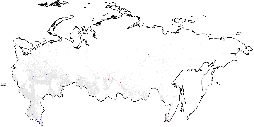
Next, I present the results from hot spot analysis of Russian 2012 elections based on the statistic computed using multiple election forensics indicators. The maps display the “hotspots” of anomalies, indicating whether the mean of values geographically close to a particular observation differs from the overall mean. The red spots in Figure 1(a) indicate whether there are clusters of atypically high values, i.e. locations where the local mean of the variable of interest is significantly greater than the overall mean value \(\bar{f}_i=0.08\). Many red spots are clumped together geographically in predominantly ethnic regions, such as Tatarstan, Bashkortostan, Mordoviya, Chuvashiya, Dagestan, Chechnya, as well as some Russian oblasts: Belgorodskaya and Voronezhskaya oblasts and several others, indicating high levels of incremental fraud probabilities. Detailed information on the number of territories and precincts belonging to anomalous clusters is provided in Table A1 of Appendix A. The predominance of blue colored spots, indicating local average scores being significantly below the overall average, are noticeably concentrated in the Moscow region and the capital.
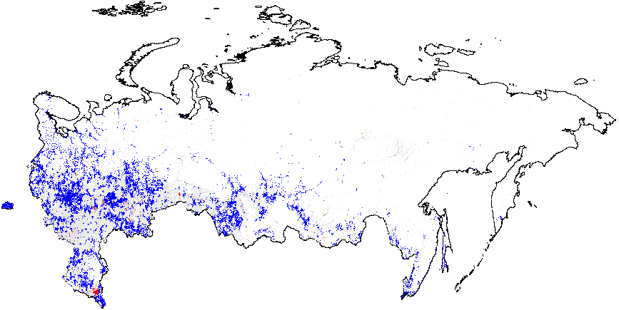
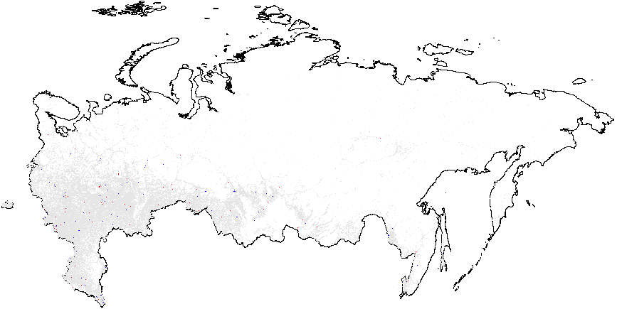
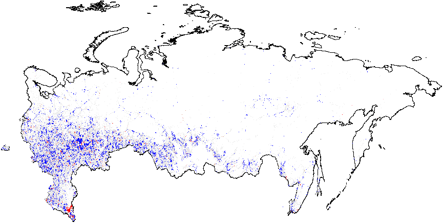
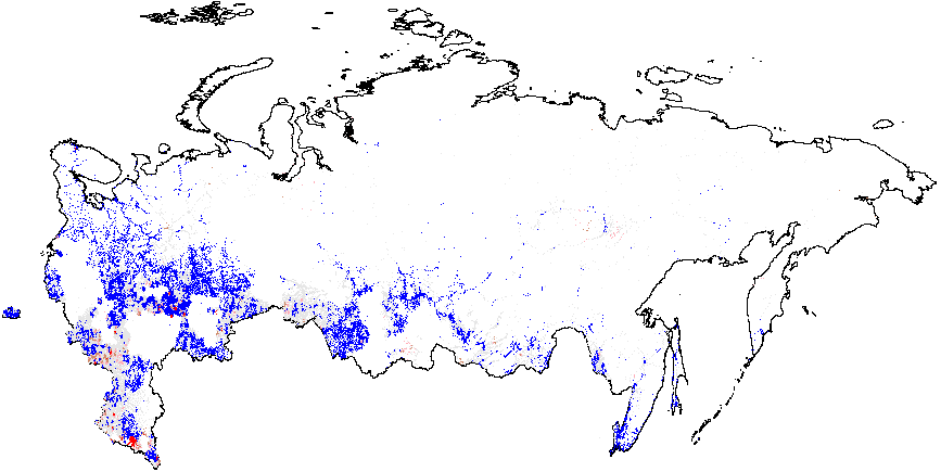
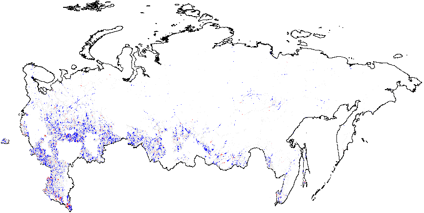
Figure 1(b) illustrates that the clusters of extreme fraud significantly higher than the global mean are mostly located in Chechnya and in the northern part of Dagestan, with smaller clusters located in Tatarstan. While Figure 1(c) does not show much evidence of localized anomalies in Putin’s vote counts {CL} against the global mean \(\overline{CL}=4.48\), as it is in close proximity to theoretical expectation, Figure 1(d) demonstrates tiny clusters scattered around the blue background with the clumps of red points located in the northern part of Dagestan (all compared to the global mean of \(\overline{P05}=0.21\)). Anomalies in turnout display similar findings. In Figure 1(e), a small blue cluster is noticeable in the Tatarstan region. However, in Figure 1, the global mean is elevated, informing us that anomalies of turnout are widespread in Russia. In this sense, Tatarstan looks uniquely “deflated”. Finally, Figure 1(f) shows that red-colored signaling patterns occur in mostly Tatarstan and in the southern Dagestan exceed the global mean of \(\overline{P05}=0.22\).
My findings for 2011 demonstrate that the geographical patterns of election forensics yield surprising consistency across both studied elections (See Figure A2 in Appendix A).
As we earlier hypothesized, across different years the clustering patterns are located in a subset of listed regions, such as Dagestan Republic, Tatarstan Republic, Belgorodskaya oblast, Bashkortostan Republic, Severnaya Osetiya Republic, Kabardino-Balkariya Republic, Mordoviya Republic, and, finally, Chechnya Republic. For several regions the finite mixture estimator is in some disagreement with the democracy scores, these regions are Chuvashskaya Republic and Voronezhskaya oblast. The finite mixture figures also demonstrate tiny dispersed clusters, which can be attributed to local political machines producing rigged election outcomes.
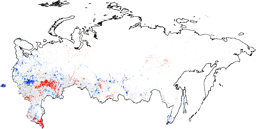
Figure 1: Hotspot and Cluster Outlier Analysis of Forensics Indicators, Russia 2012, Getis-Ord \(G_i\), Precinct-Level Data. Measures of anomalies: {P05} – 0s and 5s in the last digit of the turnout percentage and incumbent’s vote percentage; {CL} – last digits in vote counts and turnout. Overall fraud probability averages are in parentheses. (a) – \(f_i\) (0.08);
(b) – \(f_e\) (0.002);
(c) – Putin{CL}(4.48);
(d) – Putin{P05} (0.21);
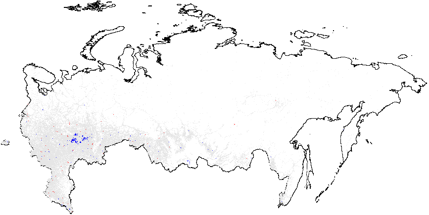
(e) – Turnout{CL} (4.939);
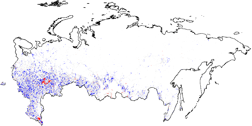
(f) –Turnout{P05} (0.22).
The next question addressed here relates to the check in geographical consistency between explored geovalues: if empirical association between these values exists than a signaling mechanism of election fraud behind the finite mixture estimates can be uncovered [25]. Figures 2 (a), (b) contain correlation matrices between respective geovalues. The categorical variable was coded by assigning to each of the precinct categories different numeric code. In the cluster analysis we deal with four basic categories of precincts: “HH” – high value among high values of anomalies; “LL” – low value among low values of anomalies; “LH” – low value among high values anomalies; “HL” – high value among low values of anomalies) measured at \(\alpha\) = 0.01 or \(\alpha\) = 0.05 significance levels. The obtained categorical variable, which will be utilized in my correlation analysis, was coded as “-2” – LL,“-1” – HL, “0” – not significant, “1” – LH and “2” – HH. The rationale for building the variable’s scale starting with cluster’s low value among low values and ending with high value among high values is to express the relative strength of clustered election fraud across the precincts.
Our findings demonstrate that for both elections the correlations between the clusters associated with signaling patterns {P05} in Putin’s/United Russia’s vote shares and signaling patterns in Turnout {P05} (\(\rho\) = 0.86 for 2011 elections; \(\rho\) = 0.91 for 2012 elections), on the one hand, as well as between estimated incremental \(f_i\) and extreme frauds \(f_e\), on the other hand, are specifically strong (\(\rho\) = 0.67 for 2011 elections; \(\rho\) = 0.77 for 2012 elections). While moderate correlation is observed between the clusters indicating extreme fraud and {P05} in turnout (\(\rho\) = 0.41 for 2011 elections; \(\rho\) = 0.45 for 2012 elections) and UR’s/Putin’s electoral support (\(\rho\) = 0.42 for 2011 elections; \(\rho\) = 0.46 for 2012 elections), quite weak correlation persists between incremental fraud and our {P05} indicator for UR’s/Putin’s electoral support(\(\rho\) = 0.28 for 2011 elections; \(\rho\) = 0.29 for 2012 elections) and turnout(\(\rho\) = 0.27 for 2011 elections; \(\rho\) = 0.25 for 2012 elections). This finding demonstrates that the geographic distribution of the finite mixture fraud probabilities can be also connected to the strength of political machines in the regions. Moreover, this finding is also backed by our expert evidence, showing that the list of the regions with the least democracy scores and strongest political machines matches partially matches the clusters of the finite mixture fraud probabilities.
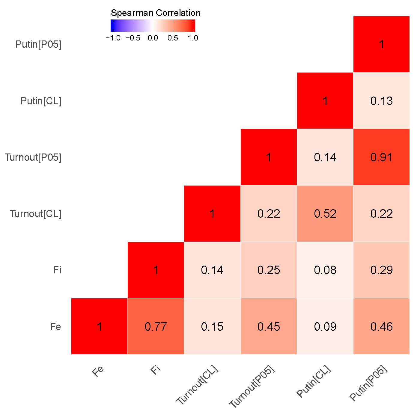
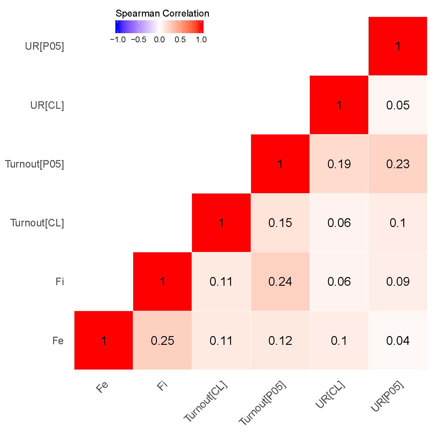
Figure 2: Correlation Matrices for Precinct-Level Data, Getis-Ord \(G_i\). (a) – 2012 presidential elections;
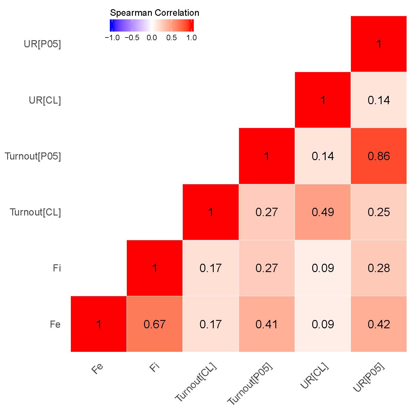
(b) – 2011 parliamentary elections.
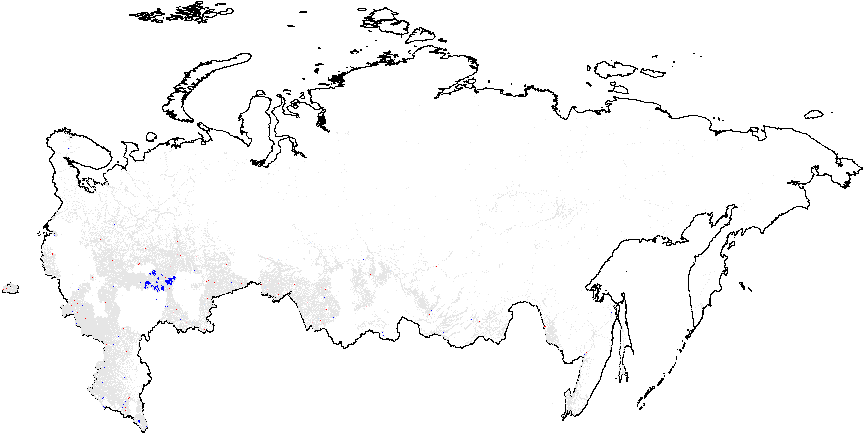
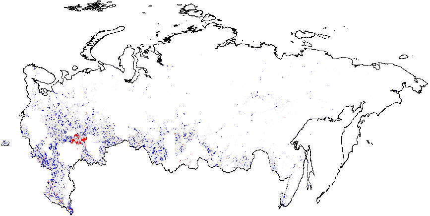
On the next stage I employ hot spot analysis of Russian elections, by calculating the mean of precinct-level election forensics indicators for each territory, i.e. subregional administrative unit. This approach enables us to test if territory-level clusters in any particular way correlate with the findings based on the precinct-level data analysis. It also helps to test the hypothesis if the likelihood of election fraud can be attributed to the territorial level. To dismiss the areas with low population density, here I intentionally present the map of western part of Russia for both estimated finite mixture measures.
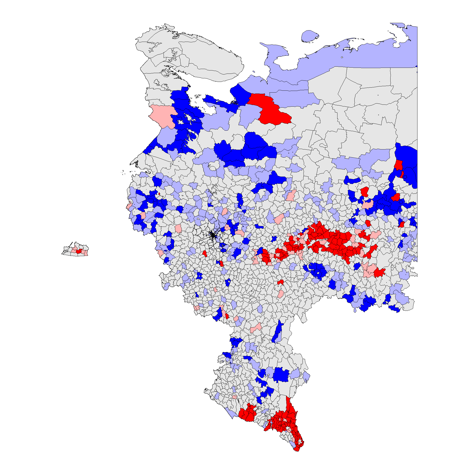
Figure 3: Cluster and Outlier Analysis for Russia 2011, 2012, \(f_i\) , local Moran’s \(I\), Territory-Level Data. Overall fraud probability averages are in parentheses. (a) – \(f_i\) 2012 (0.09);
(b) – \(f_i\) 2011(0.13);
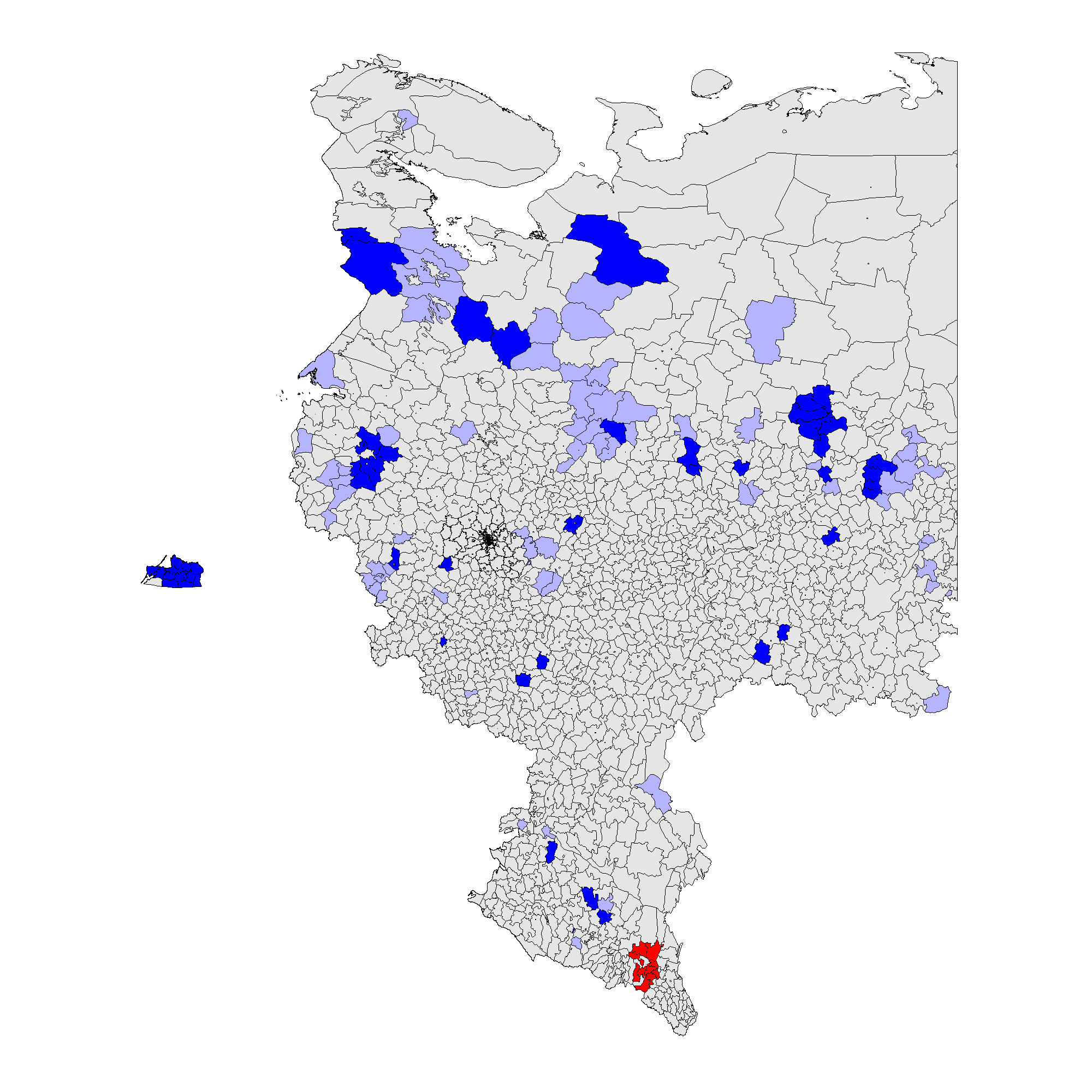
(c) – \(f_e\) 2012 (0.002);
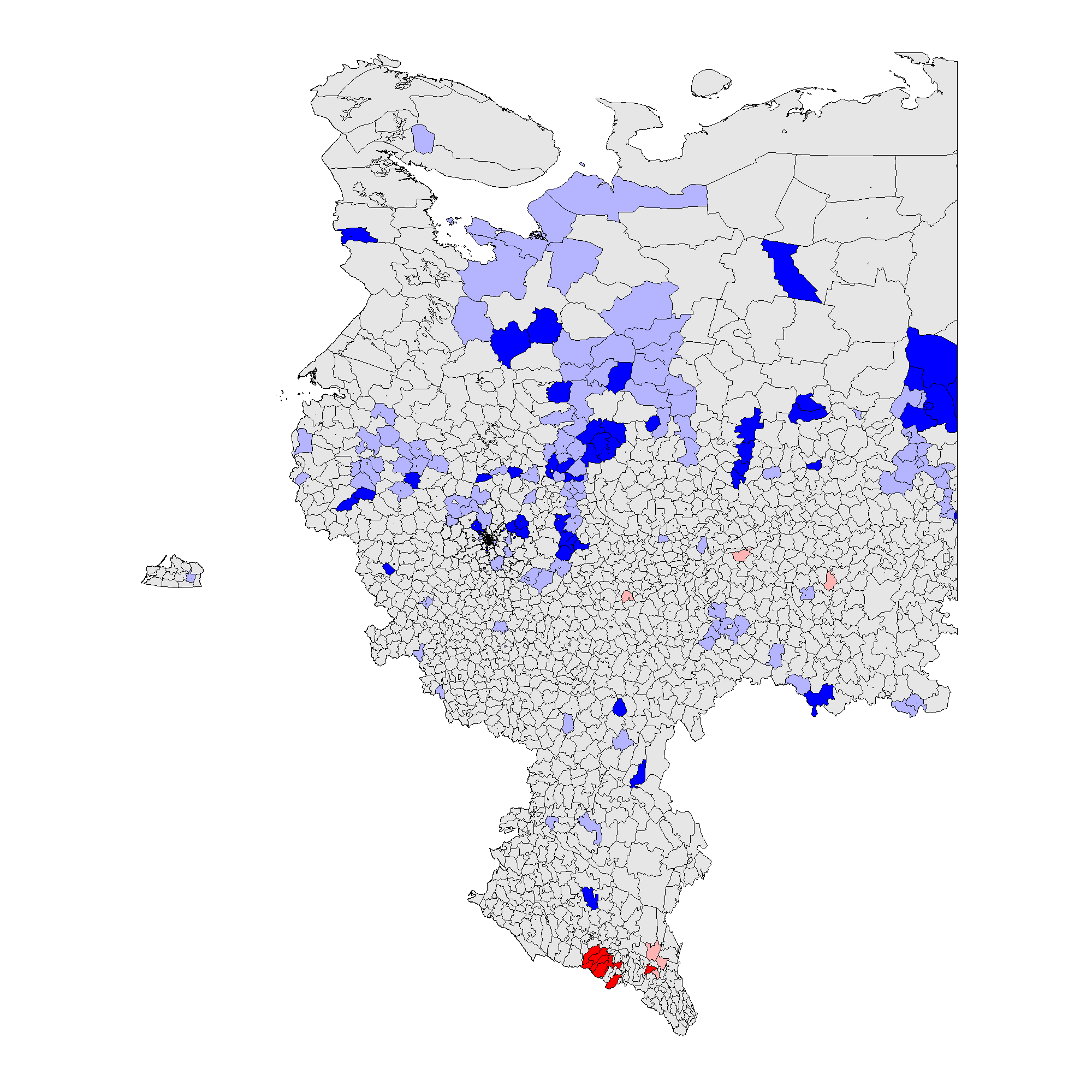
(d) – \(f_e\) 2011 (0.003).
Figure 3 shows that the patterns associated with the territory-level analysis are similar to the patterns from the precinct-level analysis. In 2012 clusters of incremental frauds \(f_i\) are persistent predominantly in ethnic territories of Tatarstan, Bashkortostan, Mordoviya, Chuvashiya, Dagestan, Chechnya, Severnaya Osetiya, and of extreme fraud \(f_e\), in Chechnya and Dagestan. In 2011 clusters of incremental fraud \(f_i\) are more dispersed involving, in addition to the previously mentioned regions, Amurskaya, Belgorodskaya, Voronezhskaya oblasts, Krasnodarskiy kray, and Karachaevo-Cherkessiya Republic and several others. Extreme fraud \(f_e\) was still prevalent in the north of Chechnya and Dagestan Republics. Moreover, since the global mean for 2011 election is elevated compared to 2012, these results indicate the presence of less heterogeneity at higher levels of electoral anomalies. For more information on the number of territories and precincts belonging to anomalous clusters check Table A1 in Appendix A.
Thus, taking into the account the totality of evidence, our Hypothesis 2 is partly confirmed by our empirical findings: the geographic clustering tests, indeed, expose the presence of election fraud clusters mainly located in the areas exhibiting poor democratic environment and the presence of the strong political machines, these are mainly the Republics and the rural territories.
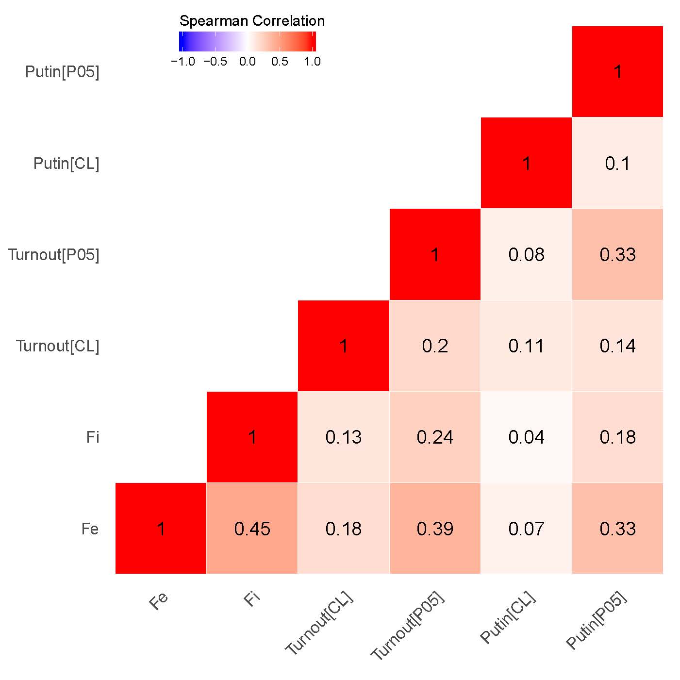
Figure 4: Correlation Matrices for Territory-Level Data, local Moran’s \(I\). (a) – 2012 presidential elections;
(b) – 2011 parliamentary elections.
Unsurprisingly, the correlation matrix built using territory-level data demonstrates somewhat weaker findings compared to the point-data correlation matrix. Notably, the correlations between the estimates of interest for the presidential elections are stronger compared to the parliamentary elections. Both finite mixture estimates weakly or moderately correlate between each other (\(\rho\) = 0.25 for 2011 elections; \(\rho\) = 0.45 for 2012 elections) and the signaling estimate {P05} (\(f_i\): \(\rho\) = 0,24 for 2011 and 2012 elections; \(f_e\): \(\rho\) = 0,12 for 2011 elections, \(\rho\) = 0,39 for 2012 elections). A moderate correlation seems to occur in 2012 between the estimates measuring signaling patterns {P05} for turnout and Putin’s support (\(\rho\) = 0.33).
Hence, the cluster analysis enables us to conclude certain anomalous data patterns in finite mixture estimates are well-captured by the last-digit election forensics measures. The observed correlation between both finite mixture estimates and signaling indicators {P05} depending on the aggregation level is moderately strong. Moreover, the territory-level anomalies seem to replicate the anomalies from the precinct level quite well. This peculiar finding yields two important derivations. First, with regard to the mechanism we can conclude that in selected territories election fraud definitely has been organized and coordinated not so much at the precinct-level, but rather at the higher levels of election commissions. Second, the lack of precise geographic information about polling stations, namely the absence of precincts coordinates, does not necessarily preclude us from performing cluster analysis at the territory level; the severity of election fraud at the level of polling stations is evident at the territory level as well.
Thus, empirical analysis is supportive of Hypothesis 3 as well: depending on the electoral context, we observe moderate or strong correlations between the geographic clusters of the final mixture estimates and the geographic clusters of forensics measures associated with signaling patterns ({P05} test for turnout and incumbent), as well as anomalous last digits in vote counts {CL} found at the levels of both precincts and territories. Hence here we can conclude that the estimates derived from the finite mixture estimator can be associated with the subnational agent’s success in mobilizing his regional political machine to provide necessary electoral support for the Kremlin’s candidate or a party.
7. Conclusion
Even though none of the election forensics statistics provide definitive proof of fraud, the combination of the data from observers and consideration of technological factors, along with the various election forensics measures enables us to strengthen our conjectures. This research has been specifically aimed at validating an innovative election forensics tool, such as the finite mixture estimator, by engaging alternative data from election observation, different voting modes and several election forensics measures sensitive to machine politics in the regions and local areas. All three hypotheses have been fully or partially confirmed by my data analysis. New measures of election fraud confirm our expectations about vote rigging taking place in the polling stations with ballot boxes rather than KOIBs, and without well-trained observers rather than with them. The use of KEGs in remote areas is associated with the lack of proper election observation and elevated likelihood of electoral malfeasance – the finite mixture estimator catches this device’s feature really well.
Our geographic clustering analysis exposes the presence of clusters mainly located in the areas exhibiting poor democratic climate with strong political machines – these are mainly the Republics and the rural territories. In addition to this, based on the presented evidence, it can be also concluded that our last-digit election forensics indicators can serve as relatively good geo-predictors of the clusters of these new measures.
Hence, as of now the development of a new election forensics estimator as a part of the Election Forensics Toolkit seems to be very promising, but surely, this new estimator has to be further validated across various electoral, political and sociocultural contexts.
Appendix. Tables and Figures

Figure A1: KEGs vs. KOIBs. Images are taken from http://www.cikrf.ru. (a) KEGs;

(b) KOIBs.
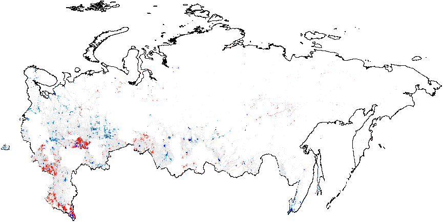
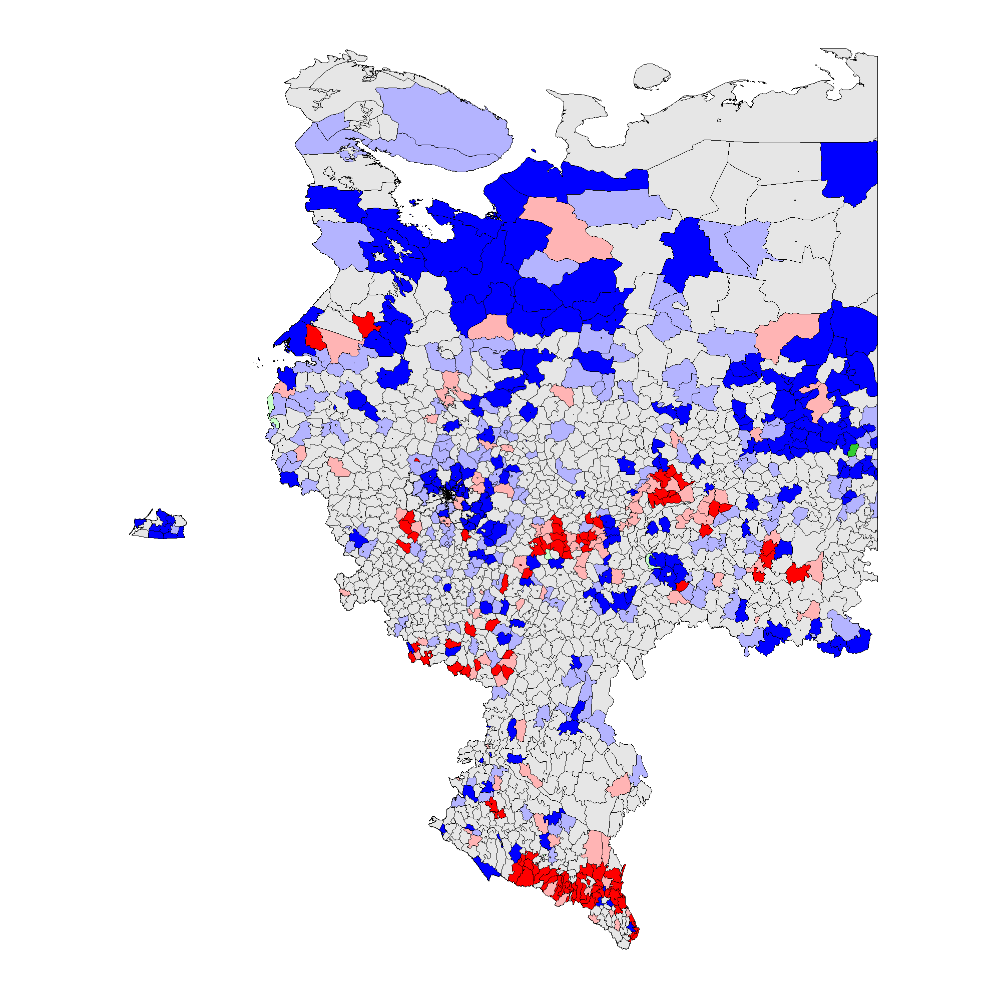
Figure A2: Hotspot and Cluster Outlier Analysis of Forensics Indicators, Russia 2011, Getis-Ord \(G_i\), Precinct-Level Data. Since some of the regions changed enumeration of their precincts between the elections in 2012 for which the geodata is available) compared to 2011 (for which there is insufficient geo data), I removed those regions from my 2011 clustering analysis. As a result, omitted regions are visible as blank spots on 2011 maps. Measures of anomalies: {P05} – 0s and 5s in the last digit of the turnout percentage and incumbent’s vote percentage; {CL} – last digits in vote counts and turnout. Overall fraud probability averages are in parentheses. (a) – \(f_i\) (0.11);
(b) – \(f_e\) (0.002);
(c) – UR{CL} (4.47);
(d) –UR{P05} (0.21);
(e) – Turnout{CL} (4.92);
(f) –Turnout{P05} (0.22).
Table A1: Number of Territories and Precincts in the Anomalous Clusters (red spots), by Region
| Region | Presidential Election | Parliamentary Election | ||||||
| Precincts | Territories | Precincts | Territories | |||||
 |
 |
|
|
|
|
|
|
|
| Amurskaya oblast | 3 | |||||||
| Belgorodskaya oblast | 4 | 171 | 2 | 17 | 280 | 14 | ||
| Bryanskaya oblast | 7 | 11 | ||||||
| Chechnya Republic | 95 | 154 | 12 | 14 | 12 | 14 | ||
| Chelyabinskaya oblast | 9 | 38 | ||||||
| Chukotskiy autonomous okrug | 1 | |||||||
| Chuvashiya Republic | 8 | 306 | 9 | 2 | 24 | 2 | ||
| Gorod Moskva | 3 | |||||||
| Irkutskaya oblast | 3 | |||||||
| Kabardino-Balkariya Republic | 162 | 179 | 8 | |||||
| Kaluzhskaya oblast | 17 | 53 | 3 | |||||
| Karachaevo-Cherkessiya Republic | 111 | 9 | 23 | 133 | 9 | |||
| Kemerovskaya oblast | 2 | 189 | 5 | |||||
| Khabarovskiy kray | 1 | |||||||
| Khanty-Mansiysk autonomous okrug | 13 | 1 | ||||||
| Kirovskaya oblast | 3 | |||||||
| Kostromskaya oblast | 1 | |||||||
The table is not fully displayed Show table
Received 25.04.2018, revision received 01.10.2018.
References
- Anselin L. Local Indicators of Spatial Association. – LISA. Geographical Analysis. 1995. V. 27. No. 2. P. 93–115.
- Arbatskaya M. Skol'ko zhe v Rossii izbiratelei? (Politiko-geograficheskii analiz obschego chisla rossiiskikh izbiratelei i urovnya ikh aktivnosti. 1990-2004) [How Many Voters Are there in Russia? (Political-geographical analysis of a General Number of the Russian Voters and Level of their Activity. 1990-2004)]. Irkutsk: Institut Geografii SO RAN, 2004. (In Russ.)
- Bader M. Do New Voting Technologies Prevent Fraud? Evidence from Russia. – The USENIX Journal of Election Technology and Systems. 2013. V. 2. No. 1. P. 1–18.
- Beber B., Scacco A. What the Numbers Say: A Digit-Based Test for Election Fraud. – Political Analysis. 2012. V. 20. No. 2. P. 211–234.
- Beber B., Scacco A. What the Numbers Say: A Digit-Based Test for Election Fraud Using New Data from Nigeria. August 2008.
- Bjornlund E.C. Beyond Free and Fair: Monitoring Elections and Building Democracy. Woodrow Wilson Center Press, 2004.
- Buzin A., Lyubarev A. Prestuplenie bez nakazaniya: administrativnye tekhnologii federal'nykh vyborov 2007–2008 godov [Crime without Punishment: administrative technologies in Russian federal elections 2007-2008]. Moscow: NIKKOLO M, 2008. (In Russ.)
- Cantu F., Saiegh S.M. Fraudulent Democracy? An Analysis of Argentina’s Infamous Decade Using Supervised Machine Learning. – Political Analysis. 2011. V. 19. No. 4. P. 409–433.
- Darr B., Hesli V. Differential Voter Turnout in a Post-Communist Muslim Society: The Case of Kyrgyz Republic. – Communist and Post-Communist Studies. 2010. V. 43. No. 3. P. 309–324.
- Deckert J., Myagkov M., Ordeshook P.C. Benford’s Law and the Detection of Election Fraud. – Political Analysis. 2011. V. 19. No. 3. P. 245–268.
- Enikolopov R., Korovkin V., Petrova M., Sonin K., Zakharov A. Field Experiment Estimate of Electoral Fraud in Russian Parliamentary Elections. – Proceedings of the National Academy of Sciences of the United States of America. 2013. V. 110. No. 2. P. 448–452.
- Estok M., Nevitte N., Cowan G. The Quick Count and Election Observation: An NDI Guide for Civic Organizations and Political Parties. Technical report, National Democratic Institute for International Affairs, 2002.
- Golosov G.V. Disproportionality by Proportional Design: Seats and Votes in Russia’s Regional Legislative Elections, December 2003–March 2005. – Europe-Asia Strudies. 2006. V. 58. No. 1. P. 25–55.
- Golosov G.V. Machine Politics: the Concept and Its Implications for Post-Soviet Studies. – Demokratizatsiya. 2013. V. 21. No. 4. P. 459–480.
- Greene K.F. Why Dominant Parties Lose. Mexico’s Democratization in Comparative Perspective. Cambridge University Press, 2007.
- Hale H.E. Correlates of Clientilism: Political Economy, Politicized Ethnicity, and PostCommunist Transition. – Patrons, Clients and Policies: Patterns of Democratic Accountability and Political Competition / Kitschelt H., Wilkinson S.I., eds. New York: Cambridge University Press, 2007. P. 227–250.
- Hale H.E. Explaining Machine Politics in Russia’s Regions: Economy, Ethnicity, and Legacy. – Post-Soviet Affairs. 2003. V. 19. No. 3. P. 228–263.
- Herron E.S. Elections and Democracy After Communism? New York: Palgrave Macmillan, 2009.
- Herron E.S. The Effect of Passive Observation Methods on Azerbaijan’s 2008 Presidential Election and 2009 Referendum. – Electoral Studies. 2010. V. 29. P. 417–424.
- Hicken A., Mebane, W.R., Jr. A Guide to Election Forensics. Working paper for IIE/USAID subaward #DFG-10-APS-UM, “Development of an Election Forensics Toolkit: Using Subnational Data to Detect Anomalies”, 2015.
- Hyde S.D. Election Fraud: Detecting and Deterring Electoral Manipulation. Washington, DC: Brookings Institution Press, 2008. P. 201–215.
- Hyde S.D. The Observer Effect in International Politics: Evidence from a Natural Experiment. – World Politics. 2007. V. 60. P. 37–63.
- Hyde S.D. The Pseudo-Democrats Dilemma: Why Election Monitoring Became an International Norm. Cornell University Press, 2011.
- Ichino N., Schundeln M. Deterring or Displacing Electoral Irregularities? Spillover Effects of Observers in a Randomized Field Experiment in Ghana. – The Journal of Politics. 2012. V. 74. No. 1. P. 292–307.
- Kalinin K., Mebane W.R., Jr. Understanding Electoral Frauds through Evolution of Russian Federalism: the Emergence of Signaling Loyalty. Paper prepared for the Annual Meeting of Midwest Political Science Association. Chicago, March 2013.
- Kalinin K., Mebane W.R., Jr. Worst Election Ever in Russia? Prepared for presentation at the 2017 Annual Meeting of the Midwest Political Science Association. Chicago, April 2017.
- Kalinin K., Shpilkin S. Kompleksnaya diagnostika fal'sifikatsii na rossiiskikh prezidentskikh vyborakh 2012 goda [Complex diagnostics of falsifications in the Russian presidential elections of 2012]. – Troitskii variant, 27.03.2012. (In Russ.) URL: http://trv-science.ru/2012/03/27/shpilkin-kalinin/ (accessed 03.03.2019). - http://trv-science.ru/2012/03/27/shpilkin-kalinin/
- Kelley J. Monitoring Democracy: When International Election Observation Works and Why it Often Fails. Princeton: Princeton University Press, 2012.
- Kireev A. Moya otsenka urovnya fal'sifikatsii na vyborakh v Gosdumu po sub'ektam federatsii [My assessment of the level of falsifications in the elections to the State Duma by subjects of the Federation]. – Livejournal, 09.10.2016. (in Russ.). URL: http://kireev.livejournal.com/1313935.html (accessed 03.03.2019). - https://kireev.livejournal.com/1313935.html
- Klimek P., Yegorov Y., Hanel R., Thurner S. Statistical Detection of Systematic Election Irregularities. – Proceedings of the National Academy of Sciences of the United States of America. 2012. V. 109. No. 41. P. 16469–16473.
- Kobak D., Shpilkin S., Pshenichnikov M.S. Statistical Anomalies in 2011-2012 Russian Elections Revealed by 2D Correlation Analysis. May 2012.
- Kuenzi M., Lambright G.M. Who Votes in Africa? An Examination of Electoral Participation in 10 African Countries. – Party Politics. 2011. V. 17. No. 6. P. 767–799.
- Magaloni B. Voting for Autocracy: Hegemonic Party Survival and its Demise in Mexico. Cambridge Studies in Comparative Politics, 2006.
- Matsuzato K. Progressive North, Conservative South? Reading the Regional Elite as a Key to Russian Electoral Puzzles. In Regions: A Prism to View the Slavic Eurasian World. Sapporo: Slavic Research Center, 2000.
- McLachlan G., Peel D. Finite Mixture Models. New York: Wiley, 2000.
- Mebane W.R., Jr. Comment on “Benford’s Law and the Detection of Election Fraud”. – Political Analysis. 2011. V. 19. No. 3. P. 269–272.
- Mebane W.R., Jr. Election Forensics: Frauds Tests and Observation-level Frauds Probabilities. Prepared for presentation at the 2016 Annual Meeting of the Midwest Political Science Association, Chicago, April 7–10, 2016.
- Mebane W.R., Jr. Election Forensics: Vote Counts and Benford’s Law. Paper prepared for the 2006 Summer Meeting of the Political Methodology Society, UC-Davis, July 20-22, 2006.
- Mebane W.R., Jr. Election Fraud or Strategic Voting? 2010.
- Mebane W.R., Jr., Kalinin K. Comparative Election Fraud Detection. Prepared for presentation at the Annual Meeting of the American Political Science Association, Toronto, Canada, Sept. 3-6 2009.
- Mebane W.R., Jr., Klaver J. Election Forensics: Strategies versus Election Frauds in Germany. Prepared for presentation at the 2015 Annual Conference of the European Political Science Association, Vienna, Austria, 2015.
- Mebane W.R., Jr. Second-digit Tests for Voters Election Strategies and Election Fraud. Prepared for presentation at the 2012 Annual Meeting of the Midwest Political Science Association, Chicago, April 12–15, 2012, April 2012.
- Mebane W.R., Jr., Sekhon J.S. Genetic Optimization Using Derivatives: The rgenoud Package for R. – Journal of Statistical Software. 2011. V. 42. No. 11. P. 1–26.
- Myagkov M., Ordeshook P.C., Shakin D. The Forensics of Election Fraud: With Applications to Russia and Ukraine. New York: Cambridge University Press, 2009.
- Norden L.., Burstein A., Hall J.L., Chen M. Post-election Audits: Restoring Trust in Elections. Technical report, Brennan Center for Justice at New York University School of Law, the Samuelson Law, Technology & Public Policy Clinic at the University of California, Berkeley School of Law (Boalt Hall), 2007.
- Ord J.K., Getis A. Local Spatial Autocorrelation Statistics: Distributional Issues and an Application. – Geographical Analysis. 1995. V. 27. P. 286–306.
- Pericchi L.R., Torres D. Quick Anomaly Detection by the Newcomb-Benford Law, with Applications to Electoral Processes Data from the USA, Puerto Rico and Venezuela. – Statistical Science. 2011. V. 26. No. 4. P. 502–516.
- Petrov N., Titkov A. Reiting Demokratichnosti Regionov Moskovskogo Tsentra Karnegi: 10 Let v Stroyu [Rating democratic regions of the Moscow Carnegie center: 10 years in the ranks]. Carnegie Moscow Center, January 2013. (In Russ.)
- Reisinger W.M., Moraski B.J. The Regional Roots of Russia’s Political Regime. Ann Arbor: University of Michigan Press, 2017.
- Sekhon J.S. Multivariate and Propensity Score Matching Software with Automated Balance Optimization. – Journal of Statistical Software. 2012. V. 42. P. 1–52.
- Shpilkin S. Dvugorbaya Rossiya [Two-Humped Russia]. – Troitskii variant, 04.10.2016. (In Russ.) URL: https://trv-science.ru/2016/10/04/dvugorbaya-rossiya/ (accessed 03.03.2019). - https://trv-science.ru/2016/10/04/dvugorbaya-rossiya/
- Shpilkin S. Statistika issledovala vybory: Statisticheskii analiz vyborov v Gosdumu 2011 goda pokazyvaet vozmozhnye fal’sifikatsii [Statistics examined elections: Statistical analysis of elections to the State Duma in 2011 indicates possible fraud]. – Gazeta.ru, 10.12.2011. (In Russ.) URL: https://www.gazeta.ru/science/2011/12/10_a_3922390.shtml (accessed 03.03.2019). - https://www.gazeta.ru/science/2011/12/10_a_3922390.shtml
- Simpser A. A Theory of Corrupt Elections. Working paper, 2006.
- Simpser A. Why Governments and Parties Manipulate Elections: Theory, Practice, and Implications. New York: Cambridge University Press, 2013.
- Sjoberg F.M. Autocratic Adaptation: The Strategic Use of Transparency and the Persistence of Election Fraud. – Electoral Studies. 2014. V. 33. P. 233–245.
- Sjoberg F.M. Making Vote Count: Evidence from Field Experiments about the Efficacy of Domestic Election Observation. Harriman Institute Working Paper No. 1, October 2012.
- Sobyanin А.А., Sukhovolsky V.G., Demokratiya, ogranichennaya fal'sifikatsiyami: Vybory i referendumy v Rossii v 1991-1993 gg. [Democracy limited by fraud: Elections and referendums in Russia in 1991-1993]. Moscow.: Project Group on Human Rights.1995. 268 p. (in Russ.).
- Solnick S.L. Federal Bargaining in Russia. – East European Constitutional Review. 1995. V. 4. No. 4. P. 52–58.