 Yurii G. Korgunyuk
Doctor of Political Sciences, Candidate of Historical Sciences, Institute of Scientific Information on Social Sciences of the Russian Academy of Sciences, [email protected]
New Instruments for Measuring Electoral Cleavages: from macro- to micro-level
Abstract
The article offers new tools for measuring electoral cleavages: a coefficient of the maximal range of a cleavage (\(Mc\)), a coefficient of the effective range of a cleavage (\(Ec\)), a coefficient of the politicization of a cleavage (\(Pc\)), a coefficient of the socialization of a cleavage (\(Sc\)). These tools take a new step in the study of cleavages at the micro-level, so that they allow a new look at the evolution of relationship between social positions and political preferences of a post-Soviet voter. Unlike factor analysis, these tools focus not on the variance of votes received by parties in different territories, but on percentage of the electorate covered by an electoral cleavage. The new tools made it possible to discover, in particular, that the electoral space of Russia was fragmented in the 1990-s and that the most influential cleavage (socioeconomic one) did not cover even a half of the electoral space. In the 2000-s the socioeconomic cleavage was supplanted by the authoritarian-democratic one which could significantly expand its maximum and effective ranges, but mainly at the expense of the administrative resource. Decrease in indicators of the authoritarian-democratic cleavage and growth in indicators of the socioeconomic (merged with the systemic one) in 2016 could be interpreted as an evidence that the usual administrative methods of controlling the electoral space gradually lose their effectiveness.
The study of electoral cleavages has been in a need of transition from macro- to micro-level for quite some time. The pioneer study by S. Lipset and S. Rokkan [13] was a classic example of macro approach: the cleavages were given a “bird’s-eye view,” so to speak, without using any mathematical tools and detailed calculations. More recent studies, such as monographs by A. Lijphart’s [12], S. Bartolini and P. Mair [3], etc. suggested an array of measuring methods for various cleavage parameters, although the preferences were still in favor of the characteristics describing the society and the political system on a macro level.
In this way, cleavages were mostly viewed as a conceptual construct rather than a “measurement unit.” Besides, there were multiple disagreements regarding the definition of the term “cleavage” [see 17]. Let us, without going into detail, suggest that the differences were mostly due to the generalized approach to the concept, due to viewing it on a macro level instead of the micro-level.
In the grand scheme of things, the main question the concept of cleavages is trying to answer is how a voter’s social status may predetermine their political choice. On a statistical level, this dependence is quite visible, and its degree varies not only from country to country, but from region to region inside one country. Ideally, identifying the degree of this dependence should be more of a technical question, rather than theoretical. To make this possible, however, we need to define a starting point – the very micro-level the measures are going to stem from.
This starting point can only be found in the election results, both national and regional, but only provided that the voters’ choice is political. From this standpoint, an analysis of the elections using the Proportional Representation system poses an optimal solution, meaning a situation where the votes are given to a political party rather than to an individual candidate.
Applying a “micro” definition to this level might seem strange, as on a micro-level political science traditionally refers to activities of an individual. However, each object has its own micro-level. For example, when studying galaxies, the life of a single star system is taken for a micro-level; if individual celestial bodies (such as planets, comets, asteroids) are taken as units of analysis, the research level is decreased excessively. This is precisely why there is no sense in considering individual candidates when studying cleavages, for it is the interaction between candidates that is of academic interest, and not their individual characteristics.
The social status of the voters is what mostly affects the territorial differences in what party gets the most votes. The author’s previous studies [7, 6, 11] propose a methodology that allows to identify the degree of political motivation and social conditioning behind the voters’ choice. Factor, correlation and regression (multiple linear regression) analyses are used as the basis of the methodology.
Factor analysis of the votes collected by the parties in different regions helped reveal the so-called “electoral cleavages.” It must be noted, however, that these are not the cleavages Lipset and Rokkan wrote about, but rather candidates for their position: the claim was validated only if the electoral cleavage had a political and social interpretation, and the electoral cleavage itself was reproduced in future elections.
The possibility for political interpretation of electoral cleavages was identified by comparing factor loadings of the participant parties (by means of correlation analysis) with their own factor loadings, but in political context. Factor analysis was also used to identify political cleavages, however in this case we used evaluations of a party’s position towards most polarizing issues (the position was evaluated on a scale from –5 to +5). The significant level of correlation between factor loadings in electoral and political space was reason enough to assume the political character of an electoral cleavage.
To identify the level of social conditioning of electoral cleavages, their factor scores were compared to demographic and socioeconomic indicators of the corresponding territorial units, which also underwent a preliminary factor analysis. The factor scores obtained as a result were used as research material to build regression models, in which the factor scores of electoral cleavages were the dependent variables.
Applying this methodology allowed us to confirm an earlier hypothesis (see [2], for example) stating that two major electoral cleavages (EC) are reproduced in electoral history of post-Soviet Russia: 1) “market liberals vs. social paternalists” that correlates closely with socioeconomic cleavage in political space; 2) “the government vs. the public” that correlates strongly with authoritarian-democratic political cleavage. Besides, both cleavages are connected to an array of social stratification factors, urbanization level above all. Moreover, if the socioeconomic cleavage was at the top in the 1990, at the beginning of the 21 century it was pushed to the second place by the authoritarian-democratic EC.
At the same time, applying this methodology to more generalized data that concerns regional election revealed several drawbacks. The main drawback is that factor analysis reacts to data variance first and foremost. Simply put, it identifies election participants with the largest swings in results as seen in different regions more quickly.
Taking this into account, the electoral cleavage during the 1999 legislative election was the opposition between the “Fatherland – All Russia” political bloc and CPRF on the one hand and the remaining candidates on the other. This cleavage was socially predetermined in a certain way (including its manifestations in the form of urbanization level and demographic characteristics), but was lacking any distinct political interpretation [7: 45–48]. The explanation was quite simple, in fact: the election results for both these organizations were characterized by dramatic swings in votes depending on the territory, varying from 2.2% in Magadan oblast to 88% in Ingushetiya for Fatherland – All Russia and from 1.82% in Ingushetia up to 43.3% in Lipetskaya oblast for CPRF. Furthermore, this “coalition” that did not exist in reality in the first place was stealing votes from other participants in a coordinated manner. This clearly demonstrates how the intervention of administrative resources, namely the opposing Fatherland – All Russia and Unity blocs, has left the first electoral cleavage without any ideological basis since it was impossible to identify any policy cleavages even after careful examination.
Still, was it the opposition between Fatherland – All Russia and CPRF on the one hand and other participants on the other hand that determined political content of 1999 election campaign? Unlikely. Everything seems to indicate that the leading role belonged to the second electoral cleavage between Fatherland – All Russia, Yabloko and The Union of Right Forces on the one hand and Unity, CPRF and the Communists – Labour Russia bloc on the other. This cleavage correlated strongly with socioeconomic and authoritarian-democratic political cleavages (PCs). Hence the question: are there any instruments that could help to register the transition of the leading position from the first to the second electoral cleavage? This article will focus on formulating and explaining such instruments.
Coefficients of maximal and effective range, politicization and socialization of electoral cleavages
Before we introduce the new instruments for measuring electoral cleavages, a brief description of the previously used methodology of identifying and interpreting them is in order (for more information see [7]). It must be noted, however, that “previously used” does not mean “obsolete” in this case.
First of all the basic methodology presupposes identifying the “electoral cleavages” only by applying factor analysis to the results obtained by the parties in various subordinate entities of the Federation (data obtained from the Central Election Commission of the Russian Federation (the CEC) was used). The factor analysis of the 2016 legislative election results revealed three factors with eigenvalues of more than one, the first factor being the United Russia’s opposition to the remaining candidates. The second factor was the cleavage between nominal marketers (Yabloko, Party of Growth, PARNAS, United Russia, Civilian Power) and social-paternalists (LDPR, Communists of Russia, CPRF) while the third factor was the opposition between Patriots of Russia and A Just Russia (Table 1).
Table 1. Electoral cleavages in the 2016 elections
| Variable | Factor Loadings (Unrotated) (Spreadsheet1) | ||
| Extraction: Principal components | |||
| (Marked loadings are >,700000) | |||
| Factor 1 | Factor 2 | Factor 3 | |
| Invalid | 0.588 | -0.52 | 0.028 |
| Rodina | 0.623 | 0.259 | 0.212 |
| Communists of Russia | 0.159 | -0.668 | 0.116 |
| Russian Party of Pensioners for Social Justice | 0.816 | -0.284 | -0.079 |
| United Russia | -0.881 | 0.421 | -0.001 |
| Russian Ecological Party “The Greens” | 0.892 | 0.212 | 0.087 |
| Civic Platform | 0.486 | -0.06 | -0.25 |
| LDPR | 0.513 | -0.69 | 0.035 |
| People's Freedom Party | 0.847 | 0.412 | 0.053 |
| Party of Growth | 0.676 | 0.495 | -0.023 |
| Civilian Power | 0.667 | 0.397 | -0.03 |
| Yabloko | 0.784 | 0.513 | 0.012 |
| CPRF | 0.341 | -0.536 | 0.15 |
| Patriots of Russia | 0.087 | -0.079 | 0.801 |
| A Just Russia | 0.409 | -0.274 | -0.533 |
| Expl.Var | 6.023 | 2.77 | 1.089 |
The table is not fully displayed Show table
The presence of political aspects in these electoral cleavages is detected by comparing the factor loadings of the parties in electoral and political spaces. Factor loadings in political space are calculated using factor analysis of evaluations given to the parties concerning their position on this or that issue. Three factors were identified for the 2016 political campaign (Table 2).
Table 2. Political cleavages in the 2016 elections
| Variable | Factor Loadings (Unrotated) (Spreadsheet1) | ||
| Extraction: Principal components | |||
| (Marked loadings are >,700000) | |||
| Factor 1 | Factor 2 | Factor 3 | |
| Rodina | -0.863 | 0.037 | -0.044 |
| Communists of Russia | -0.798 | 0.04 | 0.339 |
| Russian Party of Pensioners for Social Justice | -0.511 | -0.095 | -0.413 |
| United Russia | -0.344 | 0.509 | -0.602 |
| Russian Ecological Party “The Greens” | -0.635 | -0.048 | -0.525 |
| Civic Platform | -0.785 | -0.274 | -0.171 |
| LDPR | -0.776 | -0.14 | 0.189 |
| People's Freedom Party | 0.462 | -0.844 | 0.045 |
| Party of Growth | -0.377 | -0.72 | -0.204 |
| Civilian Power | -0.4 | -0.436 | -0.518 |
| Yabloko | 0.397 | -0.87 | 0.084 |
| CPRF | -0.796 | -0.06 | 0.524 |
| Patriots of Russia | -0.898 | -0.047 | 0.214 |
| A Just Russia | -0.875 | -0.041 | 0.269 |
| Expl.Var | 6.262 | 2.554 | 1.703 |
| Prp.Totl | 44.73% | 18.24% | 12.16% |
The first factor showcases the opposition of the liberal parties PARNAS and Yabloko to the remaining participants, first of all to the Patriots of Russia, Rodina, A Just Russia, Communists of Russia, CPRF, Civic Platform and LDPR. Since the issues with higher modular factor scores are in some way connected with foreign policy, Ukraine and fighting the “enemies within” (Table 3), this factor is interpreted as a cleavage between “imperialists” and “anti-imperialists.” It can also be regarded as a manifestation of systemic cleavage between the supporters of either westernized or independent Russia that occurred during all of the previous elections [7; 11].
Table 3. Issues with highest factor scores in the first cleavage during the 2016 Russian legislative election
| Rodina | CR | RPPSJ | UR | REPG | CP | LDPR | PARNAS | PG | CP | Yabloko | CPRF | PR | JR | Factor 1 | |
| Eurasian integration strengthens Russia’s position | 5 | 5 | 4 | 5 | 5 | 5 | 3 | -5 | 5 | 0 | -5 | 5 | 5 | 5 | -1.225 |
| Coup d’état in Ukraine | 5 | 5 | 0 | 5 | 5 | 5 | 5 | -5 | 5 | 0 | -5 | 5 | 5 | 5 | -1.143 |
| The country needs a harsher foreign policy | 5 | 5 | 3 | 5 | 3 | 5 | 5 | -5 | -3 | 3 | -5 | 5 | 5 | 5 | -1.105 |
| Supporting Putin | 5 | 3 | 5 | 5 | 5 | 5 | 4 | -5 | 4 | 5 | -4 | -3 | 5 | 5 | -1.055 |
| The US plays the main role in destabilizing the world | 4 | 5 | 0 | 5 | 4 | 5 | 5 | -5 | -2 | 4 | -5 | 5 | 5 | 5 | -1.037 |
| Supporting DPR and LPR | 5 | 5 | 4 | 5 | 4 | 5 | 5 | -5 | 0 | 0 | -5 | 5 | 1 | 5 | -1.014 |
| ... | ... | ... | ... | ... | ... | ... | ... | ... | ... | ... | ... | ... | ... | ... | ... |
| Raising the retirement age | -5 | -5 | -4 | -1 | 0 | -5 | -5 | 0 | -2 | 0 | -4 | -5 | -5 | -5 | 1.99 |
| Russia started the war in Ukraine | -5 | -5 | 0 | -5 | 0 | -5 | -5 | 5 | -5 | 0 | 5 | -5 | -5 | -5 | 2.135 |
| Repealing the NGO foreign agents law | -5 | -5 | 0 | -5 | -4 | -5 | -5 | 5 | 1 | 0 | 5 | -5 | -5 | -5 | 2.223 |
| Putin’s foreign policy is risky | -5 | -5 | -5 | -5 | -5 | -5 | -5 | 5 | -5 | -5 | 5 | -4 | -5 | -5 | 2.625 |
| Russia violated international law by annexing the Crimea | -5 | -5 | -5 | -5 | -5 | -5 | -5 | 5 | -4 | -5 | 5 | -5 | -5 | -5 | 2.641 |
The second factor is largely a manifestation of the cleavages between United Russia and the liberals, namely PARNAS and Yabloko, regarding the issues of managing the country (Table 4). We will refer to this type of cleavage as “authoritarian-democratic.”
Table 4. Issues with highest factor scores in the second cleavage during the 2016 Russian legislative election
| Rodina | CR | RPPSJ | UR | REPG | CP | LDPR | PARNAS | PG | CP | Yabloko | CPRF | PR | JR | Factor 1 | |
| Stopping the “optimization” of healthcare and education systems | 5 | 5 | 5 | -4 | 5 | 4 | 5 | 5 | 5 | 4 | 5 | 5 | 4 | 5 | -1.811 |
| Cancelling Platon tax system for truck drivers | 5 | 5 | 0 | -4 | 0 | 5 | 5 | 5 | 5 | 5 | 5 | 5 | 4 | 4 | -1.765 |
| Expanding the authority of representative government | 4 | 4 | 5 | -5 | 5 | 5 | 5 | 5 | 5 | 1 | 5 | 5 | 4 | 5 | -1.721 |
| Deepening economic crisis | 4 | 5 | 0 | -4 | 3 | 4 | 5 | 5 | 5 | 4 | 5 | 5 | 3 | 4 | -1.702 |
| The Central Bank and the government are failing to handle the crisis | 5 | 5 | 0 | -5 | 0 | 4 | 5 | 5 | 4 | 5 | 5 | 4 | 4 | 4 | -1.701 |
| Local authorities should stand for popular election | 4 | 0 | 0 | -4 | 0 | 5 | -3 | 5 | 5 | 5 | 5 | 5 | 5 | 5 | -1.679 |
| ... | ... | ... | ... | ... | ... | ... | ... | ... | ... | ... | ... | ... | ... | ... | ... |
| Position towards the municipal reform | -1 | 0 | 0 | 5 | 0 | -3 | -3 | -5 | -3 | -1 | -5 | -5 | -5 | -5 | 1.446 |
| Introducing government price control | 5 | 5 | 0 | -1 | 0 | -5 | 2 | -5 | -5 | -5 | -5 | 5 | 5 | 1 | 1.45 |
| Position towards Yarovaya “anti-terrorism” amendments | 3 | 0 | 0 | 5 | 0 | -3 | -4 | -5 | -5 | 0 | -5 | -4 | 0 | 4 | 1.495 |
| Position towards reforming Russian Academy of Sciences | -5 | -5 | 0 | 5 | 0 | -3 | 4 | -4 | -5 | -5 | -5 | -5 | -2 | -5 | 1.594 |
| Government response to the crisis and its effectiveness | -5 | -5 | 0 | 5 | 0 | -4 | -5 | -5 | -4 | -5 | -5 | -5 | -4 | -4 | 1.763 |
The third factor is the opposition between CPRF and Communists of Russia on the one hand and loyalist bloc headed by United Russia on the other regarding the socioeconomic issues primarily (Table 5). We will refer to this type of cleavage as “socioeconomic.”
Table 5. Issues with highest factor scores in the third cleavage during the 2016 Russian legislative election
| "Родина" | КР | РППзС | ЕР | РЭПЗ | ГП | ЛДПР | ПАРНАС | "Партия роста" | ГС | "Яблоко" | КПРФ | ПР | СР | Factor 1 | |
| Частная собственность эффективнее, чем государственная | 1 | -5 | 1 | 3 | 3 | 3 | 2 | 5 | 5 | 5 | 5 | -5 | -1 | -4 | -2.6 |
| Поддержка Путина | 5 | 3 | 5 | 5 | 5 | 5 | 4 | -5 | 4 | 5 | -4 | -3 | 5 | 5 | -2.462 |
| Вмешательство государства в экономическую сферу должно быть минимальным | 1 | -5 | 0 | 1 | 0 | -3 | -3 | 5 | 5 | 5 | 5 | -5 | -3 | -3 | -1.926 |
| Целесообразность вмешательства России в сирийский конфликт | 5 | -1 | 0 | 5 | 5 | 4 | 5 | -5 | 4 | 5 | -5 | 4 | 5 | 5 | -1.525 |
| Оправданность неполной индексации пенсий | 5 | -1 | 0 | 5 | 5 | 4 | 5 | -5 | 1 | 5 | -5 | 4 | 5 | 5 | -1.432 |
| Отношение к муниципальной реформе | -1 | 0 | 0 | 5 | 0 | -3 | -3 | -5 | -3 | -1 | -5 | -5 | -5 | -5 | -1.424 |
| ... | ... | ... | ... | ... | ... | ... | ... | ... | ... | ... | ... | ... | ... | ... | ... |
| Отказ от либеральной модели экономики | 5 | 5 | 0 | -3 | 0 | -2 | 3 | -5 | -5 | -5 | -5 | 5 | 5 | 5 | 1.582 |
| Национализация базовых отраслей экономики | -1 | 5 | 0 | -4 | 0 | -4 | 4 | -5 | -5 | -5 | -5 | 5 | 4 | 3 | 1.668 |
| Капитализм смертелен для России | 1 | 5 | 0 | -5 | -1 | -5 | 3 | -5 | -5 | -5 | -4 | 5 | 3 | 3 | 1.845 |
| Россия управляется авторитарными методами | -5 | 0 | -5 | -5 | -5 | 0 | 4 | 5 | -1 | 0 | 5 | 5 | 1 | 3 | 2.075 |
| Степень оппозиционности (самооценка) | -3 | 0 | -5 | -5 | -4 | -4 | 4 | 5 | 1 | -2 | 5 | 5 | 1 | 4 | 2.222 |
If we compare factor loadings in electoral and political spaces, we will get the following picture (Table 6): the first electoral cleavage is more closely connected with the second political (authoritarian-democratic) cleavage, the second electoral – with the first (“imperialistic”) and third (socioeconomic) political cleavages. The third EC has little correlation with any of political cleavages.
Table 6. Correlation between political and electoral cleavage during the 2016 Russian legislative election
| 1st political cleavage | 2nd political cleavage | 3rd political cleavage | |
| 1st electoral cleavage | 0.246 | -0.695 | 0.031 |
| 2nd electoral cleavage | 0.634 | -0.423 | -0.597 |
| 3rd electoral cleavage | -0.098 | 0.103 | 0.173 |
* Level of significance (p) – < 0.05
The next thing to be determined is whether the detected electoral cleavages have any social underlying causes. To determine this, we need to compare the factor scores of electoral cleavages to socio-demographic and economic characteristics of the corresponding regions. This comparison is possible not only by means of correlation analysis [18; 22; 21; 20], but also by means of regression analysis [2]. To avoid violating the methodological rule of using the correlating parameters as independent variables [15: 336], the author of this article suggests applying factor analysis to the socio-demographic and economic characteristic themselves, so that the factor scores obtained could be used in regression models [7; 6].
The regression model built for the 2016 election revealed a close connection between the first and second electoral cleavages and social stratification factors. The factor analysis of 47 socio-demographic and economic parameters from various federation subjects revealed a total of nine social stratification factors, four out of which can be given a sensible interpretation (Table 7).
Table 7. The results of factor analysis of social and demographic parameters in 2015
| Social stratification factors | Explained variance | % |
| Expl.Var | Prp.Totl | |
| 1. Urbanization level | 14.523 | 30.90% |
| 2. Demographic characteristics | 10.067 | 21.42% |
| 3. Economic autonomy | 4.358 | 9.27% |
| 4. Social welfare (state aid dependence) | 2.759 | 5.87% |
| Factor 5 | 2.062 | 4.39% |
| Factor 6 | 1.782 | 3.79% |
| Factor 7 | 1.433 | 3.05% |
| Factor 8 | 1.159 | 2.47% |
| Factor 9 | 1.069 | 2.27% |
Step-by-step multiple linear regression revealed a connection between the first electoral cleavage (“the government – the public”) and three social stratification factors at once – urbanization level, economic autonomy level and social welfare level (Table 8); the multiple regression coefficient was at 0.77. The second cleavage (“marketers – social-paternalists”) turned out to be connected to urbanization and economic autonomy only (Table 9) with the multiple regression coefficient at 0.697. There were no predictors for the third factor.
Table 8. Step-by-step regression model showing the link between the first electoral cleavage and social stratification factors
| Parameter Estimates (Spreadsheet1) | |||||||||
| Effect | Sigma-restricted parameterization | ||||||||
| Comment | Factor 1 | Factor 1 | Factor 1 | Factor 1 | -95.00% | 95.00% | Factor 1 | ||
| (B/Z/P) | Param. | Std.Err | t | p | Cnf.Lmt | Cnf.Lmt | Beta (?) | ||
| Intercept | -0.155 | 0.047 | -3.268 | 0.001 | -0.248 | -0.061 | |||
| 1. Urbanization | -0.595 | 0.056 | -10.666 | 0 | -0.705 | -0.485 | -0.644 | ||
| 2. Demographic char-s | Pooled | ||||||||
| 3. Economic autonomy | -0.072 | 0.036 | -2.026 | 0.044 | -0.143 | -0.002 | -0.118 | ||
| 4. Social welfare | 0.263 | 0.043 | 6.108 | 0 | 0.178 | 0.348 | 0.31 | ||
| Dependent | Test of SS Whole Model vs. SS Residual (Spreadsheet1) | ||||||||
| Variable | Multiple | Multiple | Adjusted | SS | df | MS | SS | df | MS |
| R | R2 | R2 | Model | Model | Model | Residual | Residual | Residual | |
| Factor 1 | 0.77 | 0.592 | 0.587 | 130.407 | 3 | 43.469 | 89.734 | 217 | 0.414 |
Table 9. Step-by-step regression model showing the link between the second electoral cleavage and social stratification factors
| Parameter Estimates (Spreadsheet1) | |||||||||
| Effect | Sigma-restricted parameterization | ||||||||
| Comment | Factor 2 | Factor 2 | Factor 2 | Factor 2 | -95.00% | 95.00% | Factor 2 | ||
| (B/Z/P) | Param. | Std.Err | t | p | Cnf.Lmt | Cnf.Lmt | Beta (?) | ||
| Intercept | -0.237 | 0.052 | -4.543 | 0 | -0.34 | -0.134 | |||
| 1. Urbanization | 0.203 | 0.06 | 3.391 | 0.001 | 0.085 | 0.32 | 0.218 | ||
| 2. Demographic char-s | Pooled | ||||||||
| 3. Economic autonomy | 0.504 | 0.04 | 12.741 | 0 | 0.426 | 0.582 | 0.821 | ||
| 4. Social welfare | Pooled | ||||||||
| Dependent | Test of SS Whole Model vs. SS Residual (Spreadsheet1) | ||||||||
| Variable | Multiple | Multiple | Adjusted | SS | df | MS | SS | df | MS |
| R | R2 | R2 | Model | Model | Model | Residual | Residual | Residual | |
| Factor 2 | 0.697 | 0.486 | 0.481 | 107.8134 | 2 | 53.907 | 114.136 | 218 | 0.524 |
.
This further demonstrates that the first two electoral cleavages are predetermined both politically and socially: the higher the share of the urban population is in the region and the more economically independent they are, the higher is the percentage of the people voting for liberals and against the “ruling party” and the social-paternalists.
Speaking about the third electoral cleavage, it does not have any political or social contents and thus can be considered a fluctuation caused by the competition between A Just Russia and Patriots of Russia for the “social-patriotic voter.” The small amount of votes received by these two parties raises the question of the weight of the electoral cleavages revealed by the factor analysis: can we measure it at least roughly? We can. There is data on the share of the overall number votes received by the party nationwide and their factor loadings point at the level of their involvement in each of the cleavages. If the vote percentage for each party is multiplied by their factor loadings, we will get a kind of coefficient of its participation in these cleavages.
Table 10 shows a system for calculating these coefficients. Columns 2-4 contain factor loadings of political parties based on three cleavages, column 5 contains the percentage of the votes received by each party while columns 6-8 contain the coefficients of parties’ participation in each of the cleavages (they are estimated in percentage as well but while saving the factor loading sign so that future calculations become easier). The lower lines of the table contain the sums of participation coefficients (with a plus or a minus sign); the last but one line contains the sum of coefficient modules thus yielding the maximal range coefficient (\(Mc\)) of each cleavage, that shows the maximum number of voters participating in this cleavage.
Table 10. The system of calculating the coefficients of maximum range (Mc) and effective range (Ec) of electoral cleavages the 2016 Russian legislative election
| 1 | 2 | 3 | 4 | 5 | 6 | 7 | 8 |
| Parties | Factor Loadings | Votes collected by parties (%) | Cleavage coefficient | ||||
| F1 | F2 | F3 | F1 | F2 | F3 | ||
| Rodina | 0.623 | 0.259 | 0.212 | 1.51 | 0.94 | 0.39 | 0.32 |
| Communists of Russia | 0.159 | -0.668 | 0.116 | 2.27 | 0.36 | -1.52 | 0.26 |
| Russian Party of Pensioners for Social Justice | 0.816 | -0.284 | -0.079 | 1.73 | 1.41 | -0.49 | -0.14 |
| United Russia | -0.881 | 0.421 | -0.001 | 54.2 | -47.77 | 22.8 | -0.07 |
| Russian Ecological Party “The Greens” | 0.892 | 0.212 | 0.087 | 0.76 | 0.68 | 0.16 | 0.07 |
| Civic Platform | 0.486 | -0.06 | -0.25 | 0.22 | 0.11 | -0.01 | -0.05 |
| LDPR | 0.513 | -0.69 | 0.035 | 13.14 | 6.74 | -9.07 | 0.46 |
| People's Freedom Party | 0.847 | 0.412 | 0.053 | 0.73 | 0.62 | 0.3 | 0.04 |
| Party of Growth | 0.676 | 0.495 | -0.023 | 1.29 | 0.87 | 0.64 | -0.03 |
| Civilian Power | 0.667 | 0.397 | -0.03 | 0.14 | 0.09 | 0.06 | 0 |
| Yabloko | 0.784 | 0.513 | 0.012 | 1.99 | 1.56 | 1.02 | 0.02 |
| CPRF | 0.341 | -0.536 | 0.15 | 13.34 | 4.55 | -7.15 | 2 |
| Patriots of Russia | 0.087 | -0.079 | 0.801 | 0.59 | 0.05 | -0.05 | 0.47 |
| A Just Russia | 0.409 | -0.274 | -0.533 | 6.22 | 2.54 | -1.7 | -3.31 |
| Positive response rates total | 20.53 | 25.36 | 3.65 | ||||
| Negative response rates total | -47.77 | -19.99 | -3.61 | ||||
| Coefficient of the maximal range of a cleavage (Mc) | 68.31 | 45.36 | 7.26 | ||||
The table is not fully displayed Show table
As a result, we have the following coefficient formula: \(Mс = \Sigma i |FLi|\), where \(i\) is the share of the votes received by each party according to the proportional system, \(|FLi|\) is a factor loading module of each party for the given cleavage. This formula is generalized, of course, and is based on the fact that the higher factor loading of a party is, the more voters gave their votes to it if we take the logic behind the specific cleavage into consideration. The formula may lack some important elements, but in this case the opportunity to compare different cleavages based on a uniform model is more important than accuracy. Perhaps formally it would be more correct to calculate this coefficient in the range between 1 and 0. However, the percentage proves to be more obvious when calculating fractions. Besides, values theoretically multiplied by 100 point at a rough estimate of the voters' percentage covered by this or that cleavage.
As can be seen from Table 10, the \(Mc\) coefficient of the third cleavage is rather small and covers around 7.26% of voters compared to 68.31% and 45.36% for the first and second cleavages respectively. This is another argument in favor of the fluctuating character of the third electoral cleavage during the 2016 elections.
Let us come back to the issue of calculating the participation coefficients of the parties in cleavages with plus and minus signs separately. This was done to see the power correlation. If one of the parties surpasses the other significantly (the first is \(Mс_{max}\), the second \(Mс_{min}\)), it is clear that a struggle for power is present. It is most likely going on the fringe of the range of a more powerful opponent, and the size of this fringe should be determined with an eye on the weakest part of the cleavage. This is due to the fact that the factor analysis takes the synchronized fluctuation of the results obtained by the parties in different regions into consideration, rather than the fluctuation range. The fluctuation range is unlikely to exceed the number of votes received by the weakest part. If in some region United Russia lost more votes than its opponents received in a certain cleavage, additional factors should be considered while trying to explain the losses. Only the part of the range that is comparable in size to the opponent’s power should be accounted for the share of this cleavage.
This is why we need to introduce a term called the effective range of an electoral cleavage. Its coefficient is calculated by multiplying the \(Mс_{min}\) parameter that determines the range of the weakest part by two: \(Ec = 2Mс_{min}\). Let us emphasize yet again that the accuracy is not as important as the difference between the coefficient values. In this way, \(Mc\) and \(Ec\) for the first electoral cleavage differ by a factor of 1.5, there is 12% difference for the second one and almost no difference for the third one.
Therefore, it can be concluded that the maximal range coefficient demonstrates the share of voters this or that electoral cleavage could hypothetically cover while the effective range coefficient demonstrates what share could be covered in actual fact. The other two instruments – the politicization (\(Pc\)) and socialization (\(Sc\)) coefficients – demonstrate the (approximate) share of the voters whose political preferences and social status determined their choice.
Table 11 demonstrates how these coefficients are calculated. Column 2 contains effective range coefficients for every EC, columns 3-5 contain correlation coefficients for the factor loadings of the parties in electoral and political spaces. By multiplying the correlation and effective range coefficients we will get the EC politicization coefficient (\(Pc = Ec |R|\), where \(|R|\) is the module of correlation coefficient between some electoral cleavage and some political cleavage). At the same time only the variants with at least the slightest correlation (\(|R|\) ≥ 0,3) are taken into consideration.
Naturally, this formula does not provide the most accurate results as well. Still, it is quite obvious that the higher the modular correlation between the factor loadings of electoral and political cleavages is, the more people voted based on their political preferences. Nothing more needs to be said, as the politicization coefficient values are not as important on their own as their dynamics and comparison.
Choosing the effective (instead of maximal) range coefficient as the component for the formula stems from the fact that the big difference between these two coefficients indicates that the voter’s choice was not purely political.
If the gap between the strongest and the weakest parts of the cleavage is too big, such result is usually predetermined by the unequal conditions for the campaign participants. Even if the election process was more or less fair, the big gap between parts of the cleavage may still be present. The explanation for this is that the majority of the electorate voted not based on their political preferences but rather “like everyone else,” like the majority. For this case there is an example of a Belarussian voter who confessed on TV that he gave his vote to V. Kebich in the first round of the 1994 presidential election and to A. Lukashenko in the second. The point of his confession was to say that he made a mistake in the first round and corrected it in the second by joining the majority.
Table 11. The system of calculating the coefficients of politicization (Pc) and socialization of electoral cleavages the 2016 Russian legislative election
| 1 | 2 | 3 | 4 | 5 | 6 | 7 | 8 | 9 | 10 |
| Electoral cleavages | Ec | Correlation with systemic political cleavage | Correlation with authoritarian-democratic political cleavage | Correlation with socioeconomic political cleavage | Pc (syst) | Pc (AD) | Pc (SE) | Squared multiple regression (R2) | Sc |
| F1 | 41.07 | 0.246 | -0.695 | 0.031 | 10.09 | 28.54 | 1.28 | 0.592 | 24.33 |
| F2 | 39.99 | 0.634 | -0.423 | -0.597 | 25.36 | 16.9 | 23.89 | 0.486 | 19.42 |
| F3 | 7.21 | -0.098 | 0.103 | 0.173 | 0.71 | 0.74 | 1.25 | 0 | 0 |
As it was mentioned before, in the case of the 2016 election a more or less significant correlation with political cleavages could only be observed in the first and second ECs. The first electoral cleavage had a significant correlation with authoritarian-democratic PC, the second correlated with all three of them, but mostly with authoritarian-democratic and socioeconomic ones (the corresponding correlation coefficients as well as the politicization coefficients taken into consideration are in bold).
The calculations reveal that the opposition between United Russia and the rest of the participants (liberals first of all) determined the choice for nearly 28.5% voters (column 7, line 3), the opposition between “imperialists” and “anti-imperialists” – for 25.4% (column 6, line 4), the opposition between communists and “marketers” loyal to the government – for 23.9% (column 8, line 4). At the same time, the authoritarian-democratic political cleavage in some way correlated with both the first and the second ECs, but the first had higher coefficient for both effective range and the correlation between electoral and political cleavages, which is why the politicization coefficient was higher with 28.54% (column 7, line 3) against 16.9% (column 7, line 4). Our preference will go to the first number since it exceeds the second one by a factor of 1.5.
When calculating the socialization coefficient we used multiple regression squares or determination coefficients (\(R^2\)) [1: 143–146]: \(Sc = Ec R^2\), where \(R^2\) is the multiple regression square that reflects the connection of each EC with the set of social stratification factors characteristic of a region. Choosing the effective range coefficient instead of the maximal one for the formula stems from the same reasons as with calculating the politicization coefficient. If we are talking about the cleavages instead of voters supporting certain political powers, it makes sense to limit the calculations within the segment of electoral space that this cleavage covers, but it should cover it not hypothetically, but in actual fact (in this case the \(Ec\) coefficient has more advantages than \(Mc\)).
Column 9 in Table 11 contains multiple regression squares for each of the electoral cleavages during the 2016 legislative elections. They maintain a strong presence in the first and second ECs, but are absent in the third. By multiplying them by the effective range coefficients we will get socialization coefficient values: 24.33% for the first electoral cleavage (we can assume that this is the percentage of the voters whose choice was predetermined by their social status) and 19.42% for the second.
To sum it up we can see that during the 2016 election no more than 29% of the voters were politically motivated and less than 25% were motivated socially. As for the rest of the electorate, their choice was neither politically nor socially predetermined, and was either an accident or influenced by administrative resources. We would like to mention once again that the estimates are not accurate and serve the comparative purpose only.
Still, there is a question of interpreting the differences between politicization and socialization coefficients of the ECs. Theoretically, if the values of these coefficients are close, we can assume that one and the same group of voters is the case in question (although it is not obligatory since there is no proof). If the politicization coefficient exceeds the socialization coefficient, it is most likely a sign of political motives of voters being more influential than their social status. If, on the contrary, the socialization coefficient exceeds the politicization one, the voter’s choice is most likely determined by their social status (and very often by administrative enforcement which is closely connected with social status) rather their political views.
Most likely it is not that simple. Many times the lack of any connection between the leading electoral cleavage – as a rule it is the opposition between the “ruling party” and the rest of the election participants – and social stratification factors is a consequence of ballot-box stuffing in favor of United Russia or electoral board’s downright attributing the highest results to it. In this case, the EC politicization coefficient may be quite high (as seen in 2011 elections, for example – this issue will be discussed below), but the question is whether it points to the electorate’s political motivation, and it is not an easy one to answer.
Using the instruments described above provides a different perspective on the electoral cleavages in post-Soviet Russia. The issue of the voter’s political choice being predetermined by their social status remains the most significant for the concept of cleavages, which is why we should not assign primary importance to electoral cleavages as the factor analysis identifies them as a pure formality. In this case, electoral cleavages may not be in fact cleavages but rather accidental fluctuations in the behavior of the voters. It appears more logical to start from political cleavages that manifest in the electoral ones, regardless of the fact which position is assigned to them in the hierarchy of the factor analysis. This does not mean, however, that their position in the hierarchy should be ignored, but when it should be taken into consideration based on maximal and effective range coefficients.
It is worth another reminder that the calculations provided in this article are rough, but their value is not in the accuracy but in the opportunity to observe the dynamics of structural changes in the cleavages and compare their configurations in different countries and regions.
Below are the results of applying the proposed instruments to describe the structure of cleavages in post-Soviet Russia (1993–2016). The following aspects were used as the basis of the described structure: the number of electoral cleavages during every election; the place occupied by this or that political cleavage (or, to be more specific, the electoral cleavage connected to it) in the EC hierarchy; coefficients of maximal and effective range, politicization and socialization.
The following source material was used for the research:
for identifying electoral cleavages – data from the CEC of Russia [19]; for identifying political cleavages – information from the “PartArchive” database which is being constantly updated since 1991 [14]; for identifying social stratification factors – data from Russian Federal State Statistics Service [16]. Starting from 2012, political space was measured annually and was timed to coincide with the autumn election. Starting from 2015 it was measured quarterly based on constant monitoring of public activities of the parties. For more information see [9; 10].
The structure of electoral cleavages during elections in post-Soviet Russia (1993–2016)
Since the new approach prioritizes the political aspect of the EC, it makes sense to take a closer look at the cleavages that formed the political space in Russia in 1993-2016. Only three types of cleavages manifested in the post-Soviet Russia: 1) socioeconomic; 2) authoritarian-democratic; 3) systemic, meaning that which concerns the direction of the country’s development [7; 11]. As opposed to the first two, systemic cleavage is not easily understood, but it is constantly identified by the factor analysis, never ranking lower than the second place in the hierarchy. It is rather difficult to interpret, but it includes ideological issues more often than the other two [7].
The hierarchy of these cleavages during the legislative elections can be seen in Table 12. As we can see, systemic cleavage occupied the first place in 1993 (most likely the residual effect of the 1980-1990s, when the question of “Are you for or against reforms?” was at the top of the political agenda) and socioeconomic and authoritarian-democratic placed second and third respectively.
Table 12. The hierarchy of political cleavages during legislative elections in post-Soviet Russia (1993–2016)
| Election campaign | 1st political cleavage | 2nd political cleavage | 3rd political cleavage |
| 1993 | Systemic | Socioeconomic | Authoritarian-democratic |
| 1995 | Socioeconomic | Systemic | Authoritarian-democratic |
| 1999 | Socioeconomic | Systemic | Authoritarian-democratic |
| 2003 | Socioeconomic | Systemic | Authoritarian-democratic |
| 2007 | Socioeconomic | Systemic | Authoritarian-democratic |
| 2011 | Socioeconomic | Systemic | Authoritarian-democratic |
| 2016 | Systemic | Authoritarian-democratic | Socioeconomic |
In 1995, the systemic political cleavage gave up its leading position to the socioeconomic one, and it remained so until 2011.
After 2011 the structure of political cleavages has started to change. In 2012 the authoritarian-democratic cleavage occupied the leading position, pushing the socioeconomic and systemic ones to the second and third places respectively. Everything seems to indicate that this happened due to the so-called “Snow Revolution” of 2011-2012 and tighter repressive legislation that followed it.
The situation repeated itself in 2013, and the systemic cleavage took the lead a year later after the Crimean Crisis. Its main characteristic was the opposition between the “imperialists” and “anti-imperialists” that continued the age-old dispute over whether Russia should step on the path of westernization or choose her own. The authoritarian-democratic and socioeconomic cleavages took the second and third places respectively. The situation remained the same during the 2016 legislative election [11].
Tables 13-14, along with Figures 1-3 demonstrate the way political cleavages manifested themselves in electoral cleavages.
In 1993-1995, the first electoral cleavage had a socioeconomic tinge to it (Table 13, Figure 1) The political space of 1993 was still largely dominated by the systemic, reformist and antireformist, cleavage, however the voters made it clear that for them these were the issues of the past, while the present had socioeconomic issues to resolve. As a result, the systemic political cleavage manifested itself only in the third electoral with very modest maximal and effective range, politicization and socialization parameters. The parties seemed to have learned the lesson as during the next election they toned down their reformist and antireformist sentiment. The political party “Democratic Choice of Russia” was the only one to retain that sentiment which eventually lead to it failing to get the 5% of the votes required to continue the race. In 1995, however, the systemic PC manifested itself in the second electoral cleavage with higher \(Mc\), \(Ec\) and \(Pc\) parameters.
Table 13. Mc, Ec, Pc and Sc parameters of socioeconomic electoral cleavage during 1993-2016 legislative elections
| Year | Number of electoral cleavages (EC) | Place of socioeconomic EC | Mc | Ec | Pc | Sc |
| Maximal range of socioeconomic EC | Effective range of socioeconomic EC | Politicization coefficient of socioeconomic EC | Socialization coefficient of socioeconomic EC | |||
| 1993 | 4 | 1 | 47.44 | 37.91 | 31.48 | 26 |
| 1995 | 4 | 1 | 41.48 | 40.68 | 32.56 | 21.64 |
| 1999 | 3 | 2 | 45.93 | 31.83 | 21.2 | 9.6 |
| 2003 | 4 | 2 | 27.44 | 27.41 | 20.29 | 12.79 |
| 2007 | 3 | 2 | 21.05 | 13.58 | 11.26 | 7.49 |
| 2011 | 2 | 2 | 26.07 | 22.8 | 19.15 | 10.88 |
| 2016 | 3 | 2 | 45.36 | 39.99 | 23.89 | 19.42 |
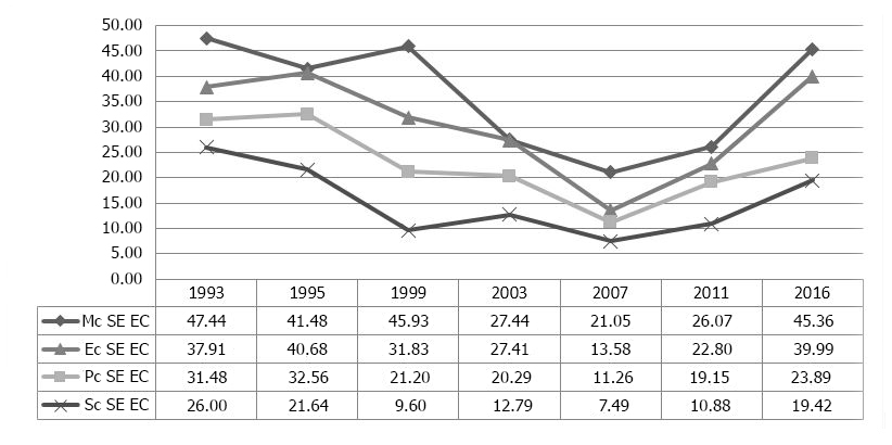
Figure 1. The dynamics of coefficients of maximal and effective range, politicization and socialization of socioeconomic electoral cleavage
In 1995, the maximal range of socioeconomic electoral cleavage decreased, while the effective range and politicization coefficient increased.
In 1999, the socioeconomic electoral cleavage placed second, but, as was said before, so did all of the political cleavages. The first EC – the opposition of CPRF and Fatherland – All Russia towards the rest of the participants – lacked any political interpretation. Having the biggest variance, the first EC still gave way to the second in terms of the maximal range coefficient – 41.37 vs 45.93, even though its effective range coefficient was higher than that of the second EC (39.32 vs. 31.83), not to mention the socialization coefficient (25.15 vs 9.6).
Coming back to our disagreement with A. Akhremenko who interpreted the first electoral cleavage as the opposition between leftist conservatives and rightist reformers (i.e. as the socioeconomic one [2: 170]), contrary to my previous assertions [7: 46-47] I have to admit that Andrei Sergeevich was not completely incorrect. It is true that the most influential cleavage (meaning the cleavage with the biggest maximal range) was socioeconomic for the most part (and authoritarian-democratic and systemic to some extent as well). The only difference was that it placed second instead of first, as was per A. Akhremenko’s assumption.
In 1999, politicization and socialization coefficient of socioeconomic cleavage decreased significantly. 21.2% of the voters were politically motivated (as opposed to 31.48% in 1993 and 32.56% in 1995) and only 9.6% were motivated socially (as opposed to 26% in 1993 and 21.64% in 1995).
During 2000s, the socioeconomic cleavage was gradually declining, albeit retaining the second place. This cleavage was at its lowest in 2007 when the maximal variance range was at 21.05, effective range was at 13.58 and politicization and socialization coefficients were at 11.26 and 7.49 respectively. Starting in 2011, its parameters began to increase gradually and in 2016 they almost reached their 1990s level (\(Mc\) at 45.36, \(Ec\) at 39.99, \(Pc\) at 23.89, \(Sc\) at 19.42); it still placed second in the hierarchy. It is worth noting, however, that such growth in 2016 was largely due to a shift in the list of participants of socioeconomic political cleavage. Whereas previously liberals were the main opponents of the communists in this PC, the former were replaced by United Russia and its satellites [11: 102]. During the first half of 2010s, the socioeconomic political cleavage was partially absorbed by the authoritarian-democratic one: the opposition on social and economic policies was not so much between the supporters of planned and market economy, but rather between critics and supporters of the government. This is precisely why liberals were drawn to the center of the opposition.
Even during the 1990s, when it dominated the political space, the socioeconomic cleavage did not cover even the half of electoral space and was in the lead largely due to the absence of any “centralized power,” whose interference into the election could shift the balance of power towards the authoritarian-democratic EC (“the government–the public”).
As the power was becoming more centralized around one party, the authoritarian-democratic cleavage was gaining strength (Table 14, Figure 2). The strengthening became apparent in 1999, when a correlation was revealed between the second electoral cleavage and all three political cleavages. Before that, the authoritarian-democratic cleavage was marginal, as it placed fourth out of four cleavages in 1993 and 1995. It was at its lowest point in 1995 with the maximal range at 13.51, the effective range at 13.39, and politicization and socialization coefficients at 5.49 and 2.24 respectively.
Table 14. Mc, Ec, Pc and Sc parameters of authoritarian-democratic electoral cleavage during 1993-2016 legislative elections
| Year | Number of electoral cleavages (EC) | Place of authoritarian-democratic EC | Mc | Ec | Pc | Sc |
| Maximal range of authoritarian-democratic EC | Effective range of authoritarian-democratic EC | Politicization coefficient of authoritarian-democratic EC | Socialization coefficient of authoritarian-democratic EC | |||
| 1993 | 4 | 4 | 26.75 | 23.89 | 16.99 | 6.11 |
| 1995 | 4 | 4 | 13.51 | 13.39 | 5.49 | 2.24 |
| 1999 | 3 | 2 | 45.93 | 31.83 | 16.68 | 9.6 |
| 2003 | 4 | 1 | 60.4 | 51.38 | 34.05 | 36.7 |
| 2007 | 3 | 1 | 86.18 | 48.95 | 35.06 | 32.41 |
| 2011 | 2 | 1 | 84.52 | 73.18 | 64.71 | 48.24 |
| 2016 | 3 | 1 | 68.31 | 41.07 | 28.54 | 24.33 |
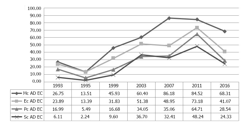
Figure 2. The dynamics of coefficients of maximal and effective range, politicization and socialization of authoritarian-democratic electoral cleavage
The “accession” of the authoritarian-democratic EC coincided with the beginning of a new century. Having occupied the top of the hierarchy in 2003, it retains this position to this day. The maximal range peak of this cleavage fell on 2007 (86.18), while the highest values for effective range, politicization and socialization coefficients (73.18, 64.71 and 48.24 respectively) fell on 2011. This was in part connected to a certain increase in competition and political struggle. In 2016 the parameters for this cleavage started to decrease, which can be identified as a downturn in social activism. Nevertheless, the authoritarian-democratic electoral cleavage is still dominant, albeit not as forcefully as before.
The systemic cleavage has been overshadowed by the stronger PCs throughout the whole post-Soviet period (Table 15, Figure 3). In the early 1990s, however, it surpassed the authoritarian-democratic cleavage while staying behind the socioeconomic one by placing third in 1993 and second in 1995. In 1999 the systemic PC found its reflection in the second electoral cleavage along with the rest of PCs, which explains the sudden increase in its parameters. From 2000 to 2010, the systemic cleavage lost its independence, usually merging with the socioeconomic one and having a lower politicization coefficient (except for the 2016 election when it went forward in this regard, which can be considered a consequence of the Kremlin’s decision to annex Crimea). Only in 2007 did this cleavage merge with authoritarian-democratic almost completely, which dramatically increased its maximal and effective range coefficients as well as the socialization one (Figure 5). The politicization coefficient changed only slightly.
Table 15. Mc, Ec, Pc and Sc parameters of systemic electoral cleavage during 1993-2016 legislative elections
| Year | Number of electoral cleavages (EC) | Place of systemic EC | Mc | Ec | Pc | Sc |
| Maximal range of systemic EC | Effective range of systemic EC | Politicization coefficient of systemic EC | Socialization coefficient of systemic EC | |||
| 1993 | 4 | 3 | 27.47 | 22.03 | 9.39 | 6.29 |
| 1995 | 4 | 2 | 27.56 | 25.61 | 13.34 | 4.75 |
| 1999 | 3 | 2 | 45.93 | 31.83 | 12.15 | 9.6 |
| 2003 | 4 | 2 | 27.44 | 27.41 | 18.85 | 12.79 |
| 2007 | 3 | 1 | 86.18 | 48.95 | 18.78 | 32.41 |
| 2011 | 2 | 2 | 26.07 | 22.8 | 19.1 | 10.88 |
| 2016 | 3 | 2 | 45.36 | 39.99 | 25.36 | 19.42 |
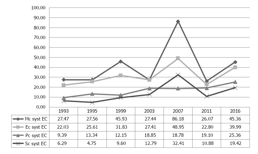
Figure 3. The dynamics of coefficients of maximal and effective range, politicization and socialization of systemic electoral cleavage
Table 16. The hierarchy of politically interpreted electoral cleavages during 1993-2016 legislative elections
| Year | Number of electoral cleavages (EC) | Place of socioeconomic EC | Place of authoritarian-democratic EC | Place of systemic EC |
| 1993 | 4 | 1 | 4 | 3 |
| 1995 | 4 | 1 | 4 | 2 |
| 1999 | 3 | 2 | 2 | 2 |
| 2003 | 4 | 2 | 1 | 2 |
| 2007 | 3 | 2 | 1 | 1 |
| 2011 | 2 | 2 | 1 | 2 |
| 2016 | 3 | 2 | 1 | 2 |
Table 16 showcases yet another difference in the structure of electoral cleavages in 1990s and 2000-2010s. In 1990s, political cleavages were spread among different ECs. In 1999 they merged in one of the cleavages – second in the hierarchy. Starting from 2003 they branched off to the different cleavages, but only partially: the systemic cleavage for one lost its independence and was bouncing back and forth from socioeconomic to authoritarian-democratic.
Table 16
To sum it up, the highly competitive conditions during 1990 elections were determined by a relatively weak government rather than a strong society. Even the most significant electoral cleavage – the socioeconomic one – covered less than half of the voters, maximal range parameter included (not to mention the rest of them). In the 2000s, the central government mobilized the majority of the electorate while making active use of administrative resources, thus ensuring the leading position for the authoritarian-democratic cleavage. The weakening of the latter in 2016 on the one hand and the strengthening of socioeconomic and systemic cleavages on the other may indicate that administrative control in electoral spaces was becoming less effective.
Conclusion
Introducing new instruments for measuring electoral cleavages, such as maximum (\(Mc\)) and effective (\(Ec\)) range coefficients as well as politicization (\(Pc\)) and socialization (\(Sc\)) coefficients, demonstrates yet another new way of studying cleavages on a micro-level. It also provides a different perspective on the evolution of the correlation between social status and political preferences of the voters in post-Soviet Russia. The earlier methodologies that utilized simple factor analysis focused mostly on the variance of votes that a party received in different regions. Many details identifying the part of the electorate covered by this or that cleavage dropped out of the research as a result.
Applying these new instruments helped identify the fragmented character of the electoral space in Russia during the 1993 and 1995 elections in particular: there was a separate electoral cleavage for every political one. Besides, even the strongest of political cleavages – the socioeconomic one – did not cover even the half of the entire electoral space.
The research also revealed that during the 1999 elections the socioeconomic cleavage, retaining the maximal range, was pushed back to the second place under the pressure of the administrative resources. Moreover, because of this pressure, all of the political cleavages – socioeconomic, authoritarian-democratic and systemic, that is – found their reflection, with varying degree of intensity, in the singular electoral cleavage, which was second in sequence.
In 2000’s, the increase of bureaucratic control over the election process and centralization of administrative resources have led to the advancement of the authoritarian-democratic political cleavage. This specific cleavage reached its peak in 2007 (maximal range coefficient) and 2011 (effective range, politicization and socialization coefficient). As opposed to socioeconomic, the authoritarian-democratic cleavage was able to cover the bigger part of the electorate, albeit due to the bureaucratic factors instead of political ones. At the same time, the socioeconomic cleavage was only pushed back to the second place and not out of the electoral space in general. Moreover, starting in 1999 there occurred a trend of political cleavages merging in various combinations in one random electoral cleavage.
The decrease of authoritarian-democratic parameters after the 2016 election campaign (and, to the contrary, the increase of socioeconomic parameters as well as systemic ones, which merged with socioeconomic) may indicate that the usual administrative control measures in electoral spaces are gradually losing their effectiveness. Future election will show whether this is true or not.
The methodology described in the article requires further improvement. Ideally, it should be tested on data from other countries that utilize the proportional electoral system. Such initiative, however, requires help from experts on country studies (the study of campaign merchandise implies not only a good command of the language, but of the political concepts specific to this or that country; otherwise it is impossible to either identify any pressing issues or evaluate the parties’ positions).
However, there is plenty of research opportunity in Russia as well, as one simply needs to level down the research from federal to regional. Despite the highly nationalized party system in the country [4, 5], Russian regions differ greatly from each other when it comes to the structure of political and electoral cleavages. The author plans to address this very issue in his future article.
Received 18.12.2017, revision received 28.06.2018.
References
- Akhremenko A.S. Politicheskii analiz i prognozirovanie: uchebnoe posobie [Political Analysis and Forecasting: A Manual]. Moscow: Gardariki, 2006. 333 p. (In Russ.)
- Akhremenko A.S. Struktura elektoral'nogo prostranstva [The Structure of the Electoral Space]. M.: Sotsial'no-politicheskaya mysl'. 2007. 320 p. (In Russ.)
- Bartolini S., Mair P. Identity, Competition, and Electoral Availability. The Stabilisation of European Electorates 1885–1985. – Cambridge: Cambridge University Press. 1990. 363 p.
- Golosov G.V., Grigor'ev I.S. Natsionalizatsiya partiinoi sistemy: rossiiskaya spetsifika [The nationalization of the party system: Russian specifiecs]. – Politicheskaya nauka. 2015. No. 1. P. 128–156. (In Russ.)
- Golosov G.V. Party system nationalization: The problems of measurement with an application to federal states. – Party Politics. 2016. V. 22. No. 3. P. 278–288.
- Korgunyuk Yu. Cleavage Theory and Elections in Post-Soviet Russia. – Perspectives on European Politics and Society. 2014. V. 15. No. 4. P. 401–415.
- Korgunyuk Yu.G. Kontseptsiya razmezhevanii i faktornyi analiz [Cleavage Theory and Factor Analysis]. – Politiya. 2013. No. 3. P. 31–51. (In Russ.)
- Korgunyuk Yu.G. Model' razmezhevanii i rossiiskie vybory: postanovka issledovatel'skoi zadachi [Cleavage Theory and Russian elections: formulation of the research problem]. – Mirovoi krizis i politicheskie izmeneniya. Politicheskaya nauka: Ezhegodnik 2009. Moscow: ROSSPEN. 2010. P. 334–372. (In Russ.)
- Korgunyuk Yu.G. Partiinaya reforma 2012–2014 gg. i struktura elektoral'nykh razmezhevanii v regionakh Rossii [The Party Reform of 2012–2014 and the Electoral Cleavage Structure in Russian Regions]. – Politicheskie issledovaniya. 2015. № 4. S. 97–113. (In Russ.)
- Korgunyuk Yu.G., Shpagin S.A. Vybory v regional'nye sobraniya 13 sentyabrya 2015 goda i izmeneniya v partiino-politicheskom prostranstve Rossii [The 13 September 2015 Elections to Regional Legislatures and Changes in the Russian Party System and Political Space]. – Politiya. 2016. No. 2(82). P. 55–76. (in Russ.)
- Korgunyuk Yu.G. Vybory po proportsional'noi sisteme kak massovyi opros obshchestvennogo mneniya [Proportional Elections as Mass Opinion Poll]. – Politicheskaya nauka. 2017. No. 1. P. 90–119. (in Russ.)
- Lijphart A. Democracies: Patterns of Majoritarian Consensus Government in Twenty-one Countries. New Haven, CT: Yale University Press. 1984. 229 p.
- Lipset S. M., Rokkan S. Cleavage Structures, Party Systems, and Voter Alignments: An Introduction. – Party Systems and Voter Alignments: Cross-National Perspectives. – New York; London: The Free Press, Collier-MacMillan limited. 1967. P. 1–64.
- PartArkhiv [Partу Archive]. – Partinform website. URL: http://www.partinform.ru/pa98 (accessed 16.02.2019). - http://www.partinform.ru/pa98
- Popova O.V. Politicheskii analiz i prognozirovanie: uchebnik [Political Analysis and Forecasting: Textbook]. Moscow: Aspekt Press, 2011. 464 p. (in Russ.)
- Regiony Rossii. Sotsial'no-ekonomicheskie pokazateli [Regions of Russia. Socio-economic indicators. – The official site of the Federal State Statistics Service. (In Russ.) URL: http://www.gks.ru/wps/wcm/connect/rosstat_main/rosstat/ru/statistics/publications/catalog/doc_1138623506156 (accessed 16.02.2019). - http://www.gks.ru/wps/wcm/connect/rosstat_main/rosstat/ru/statistics/publications/catalog/doc_1138623506156
- Römmele A. Struktura razmezhevanii i partiinye sistemy v Vostochnoi i Tsentral'noi Evrope [Cleavage Structure and Party Systems in East and Central Europe]. – Politicheskaya nauka. 2004. No. 4. P. 30–50. (In Russ.)
- Slider D., Gimpelson V. E., Chugrov S. Political Tendencies in Russia Regions — Evidence from the 1993 Parliamentary Elections. – Slavic Review. 1994. V. 53. No. 3. P. 711–732.
- Vybory, referendum i inye formy pryamogo voleizyavleniya [Elections, referendums and other forms of the direct declaration of will]. – The official website for the Central Election Committee of Russia. URL: http://www.vybory.izbirkom.ru/region/izbirkom (accessed 16.02.2019). (In Russ.) - http://www.vybory.izbirkom.ru/region/izbirkom
- Zarycki T. Four Dimensions of Center-Periphery Conflict in the Polish Electoral Geography. – Social Change. Adaptation and Resistance. Warsaw: Warsaw University — Institute for Social Studies, 2002. P. 19–38.
- Zarycki T., Nowak A. Hidden Dimensions: the Stability and Structure of Regional Political Cleavages in Poland. – Communist and Post-Communist Studies. 2000. V. 33. No. 2. P. 331–354.
- Zarycki T. The New Electoral Geography of Central Europe. – Research Support Scheme Electronic Library, Open Society Institute, Budapest, 1999. URL: http://rss.archives.ceu.hu/archive/00001080/01/80.pdf (accessed 27.10.2016). - http://rss.archives.ceu.hu/archive/00001080/01/80.pdf
- Bértoa F. C. Party systems and cleavage structures revisited: A sociological explanation of party system institutionalization in East Central Europe. – Party Politics. 2014. V. 20(1). P. 16–36.