 Yurii G. Korgunyuk
Doctor of Political Sciences, Candidate of Historical Sciences, Institute of Scientific Information on Social Sciences of the Russian Academy of Sciences, [email protected]
New Instruments for Measuring Electoral Cleavages and Regional Map of Cleavages during the 2011 and 2016 Elections
Abstract
This article is a follow-up to the "New Instruments for Measuring Electoral Cleavages: from Macro- to Micro-Level" article published in the previous issue. The article attempts to analyze the structure of regional electoral and political cleavages during the 2011 and 2016 Russian legislative elections. The corresponding regional map was created using the electoral cleavage measurement tools introduced before, namely maximal and effective range coefficients, politicization coefficient, socialization coefficient and balance ratio coefficient. The research revealed a connection between the political competitiveness level in the region and the political distinctiveness of electoral cleavages. The lower the competitiveness level, the more detailed the political landscape is from a voter's perspective and vice versa: the correlation between electoral cleavages and political dimensions in the most competitive regions often goes beyond the 5% margin of error. This trend manifested in 2011 and became more pronounced in 2016: the voters' perception of political landscape got more complicated even in the least competitive regions while the cluster of regions with the weakened correlation between electoral cleavages and political dimensions almost doubled in size. The reasons behind that were most likely the decreased administrative pressure during the elections as well as disoriented opposition voters (especially liberal-leaning ones). The former was caused by the "imperialistic vs anti-imperialistic" polarity that came to dominate the political space.
Electoral cleavage measurement tools introduced in the previous article [18] offer new insights into the differentiation of the structure of electoral cleavages from the regional standpoint.
Previous method of measuring electoral cleavages on the regional level [19; 15] has determined five clusters of regions following the 2011 legislative election: 1) least competitive – the republics of North Caucasus: Dagestan, Ingushetia, Chechnya, Kabardino-Balkaria, Karachay-Cherkessia and North Ossetia where the bureaucratic "artistry" of electoral boards completely replaced any actual electoral life; 2) moderately non-competitive – Mordovia, Mari El, Tatarstan and Tyumen Oblast where several towns managed to preserve pockets of political resistance despite full administrative resource domination, which lead to significant dispersion in voting for United Russia; 3) slightly competitive – 19 regions where the force of administrative resource was somewhat limited, leaving room for the second electoral cleavage to manifest (the following Republics: Adygea, Bashkortostan, Kalmykia, Altai, Komi and Tyva; Chukotka and Yamalo-Nenets Autonomous Okrugs; the following Oblasts: Bryansk, Voronezh, Kaluga, Kemerovo, Omsk, Oryol, Penza, Saratov, Tambov and Ulyanovsk); 4) averaged – 32 regions where election results were more dependent on the voter and their social characteristics than in the previous cluster (Moscow, Buryatia, Udmurtia, Khakassia, Chuvashia, Yakutia, Stavropol and Khabarovsk Krais; the following Oblasts: Amur, Arkhangelsk (with Nenets AO), Astrakhan, Volgograd, Irkutsk, Kaliningrad, Kursk, Lipetsk, Magadan, Nizhny Novgorod, Novosibirsk, Orenburg, Rostov, Ryazan, Samara, Smolensk, Tver, Tomsk, Tula, Chelyabinsk and Yaroslavl; Khanty-Mansi Autonomous Okrug, Jewish Autonomous Oblast); 5) most competitive – 20 regions (Saint-Petersburg, Karelia; the following Krais: Altai, Zabaykalsky, Kamchatka, Krasnoyarsk, Perm and Primorsky; the following Oblasts: Vladimir, Vologda, Ivanovo, Kirov, Kostroma, Kurgan, Leningrad, Moscow, Murmansk, Pskov, Sakhalin and Sverdlovsk) [19; 15].
Since factor analysis is primarily centered on the dispersion of party results and does not consider features like cleavage range, the Chechen Republic (Chechnya) with its 99.5% votes for United Russia fell out of focus. Even the first out of the three "cleavages" identified there displayed the effective range of 0.49 (i.e. less than half percent of electorate). As a matter of fact, cleavages in this region are virtually non-existent. At the same time, Chechnya shares the cluster with Kabardino-Balkaria where the "party of power" found a serious challenge in CPRF, which accumulated a regional average of 17.5% votes, with more than 20% in certain districts.
This shows there is certainly a need to further improve the clustering method by taking into consideration the details that fell out of its focus. The new method is intended for creating a regional map of cleavages following the 2011 and 2016 legislative elections.
Research method
Before moving on to the new research method, we shall give a brief overview of its differences from the old one, because the new method does not overrule the old but rather corrects and expands it.
Let us recall that both new and old method are based on the so-called "electoral cleavages" that are calculated through factor analysis of the results gained by the parties in various territorial units.
These are obviously not the "cleavages" Lipset, Rokkan and their numerous followers describe [24; 23; 3, etc.]. In our research, cleavages are inter-territorial differentiation factors for votes casted for different parties under the proportional representation system, i.e. they are more like applicants to the Lipset-Rokkan cleavages: the claims are justified only if the electoral cleavages appear to have a political interpretation and social connotations and the cleavages themselves regularly manifest in subsequent elections.
The possibility of electoral cleavages having a political interpretation is revealed through comparing factor loadings of parties participating in the elections with factor loadings of the same parties in a political space. Correlation analysis is used for such a comparison.
There are many ways to reveal the political content of a cleavage: expert surveys [11; 27; 33], elite and mass surveys [13; 22] content analysis of party platforms [6; 5] or a combination of these methods [2]. All these ways have their own advantages and disadvantages. We attempted to put forward our own method of revealing these overtones based on constant monitoring of the views of the parties on the most polarizing issues [16; 20; 18; 14]. These views were evaluated on a scale from –5 to +5 and subjected to factor analysis as well. The resulting factors were defined as political cleavages [16; 20; 18; 14].
Three such political cleavages have been identified in post-Soviet Russian elections: 1) the traditional socioeconomic (left-right) cleavage, which is usually identified through content analysis developed by Ian Budge and his followers; 2) authoritarian-democratic cleavage which is not exactly relevant for Europe, but quite wide-spread in post-Soviet states and Latin America [1; 31; 29: 32]; 3) systemic cleavage which manifests as opposition between proponents of open and closed societies.
This openness/closedness may both be of temporal and spatial quality. In the former case the opponents focus on the future/past while in the latter they focus on supranational organizations integration or, on the contrary, isolationism. The "temporal" variation of systemic cleavage can be observed in the opposition between materialists and postmaterialists [12], new and old politics [7; 25]. The "spacial" variation can in its turn be observed in the opposition between demarcationists and integrationists (i.e. those who benefited from globalization and those who did not) [21], universalists and particularists [8], cosmopolites and communitarianists [30]. Last but not least, combined variations oppose libertarian-universalists to traditionalist-communitarianists [4] or Green/alternativists/libertarians to traditionalists/authoritarians/nationalists (GAL/TAN) [10; 9].
A relatively strong correlation between factor loadings of parties in electoral and political space suggests that this or that electoral cleavage has a political interpretation.
A correlation analysis confirmed the previous suggestion (see [1] for example) that the electoral history of post-Soviet Russia reveals constant re-runs of two main electoral cleavages (EC): 1) "liberal marketeers vs social paternalists" that is closely correlated with socioeconomic cleavage in political space; 2) "government vs the general public" that is closely correlated with authoritarian-democratic political cleavage. What is interesting is that the socioeconomic cleavage was the one dominating the landscape in the 1990s, the beginning of the 21st century saw it pushed into the background by the authoritarian-democratic cleavage.
To determine the social subtext of electoral cleavages, their factor scores were supposed to be compared to demographic and socioeconomic parameters of the corresponding territorial units.
As a rule, such comparison was made by means of correlation [28; 36; 35; 34] and regression analyses [1]. To avoid defying the methodological ban on using correlating parameters as independent variables [26], it was proposed to subject the socio-demographic and economic characteristics per se to the analysis and then to use the resulting factor scores in regression models [16; 14].
A stepwise multiple linear regression (OLS model) revealed there was a connection between "government vs the general public" and "marketeers–social paternalists" electoral cleavages and several inter-regional differentiation factors. By and large, these factors demonstrated the stratification of Russian society based on several characteristics: above all, the quality of life (generally equivalent to the level of urbanization) as well as the level of economic independence and social well-being. During the 2011 election, demographic characteristics were on this list as well.
The following was considered while clustering the regions of Russia: coefficients of correlation between factor loadings of electoral and political cleavages (modulo); modules of beta-coefficients in regression models of connection between EC and trans-regional differentiation factors. Some other aspects taken into consideration were voter turnout in every region, correlation coefficient between turnout and voting for United Russia, the number of electoral cleavages in the given region (namely the amount of explained variance for each cleavage).
This is the essence of the previous clustering method. The new method is based on using electoral cleavage measurement tools that were introduced in the previous article [18]. Let us recall that these are maximum range and effective range coefficients as well as politicization and socialization coefficients for ECs that are calculated according to the following formulae:
maximum range coefficient formula: \(Mс = \Sigma i |FLi|\), where \(Mc\) is the electoral cleavage maximum range coefficient, \(i\) is the share of votes received by each party under the proportional representation system and \(|FLi|\) is the factor loading for each party on the given cleavage;
effective range coefficient formula: \(Ec = 2Mс_{min} \), where \(Mс_{min}\) is the range of the weaker part of the cleavage;
politicization coefficient formula: \(Pc = Ec |R|\), where \(|R|\) is the module of correlation coefficient of some electoral cleavage with some political cleavage;
socialization coefficient formula: \(Sc = Ec R^2\), where \(R^2\) is a squared multiple regression (coefficient of determination) that reflects the connection of each EC with a set of inter-territorial differentiation factors typical for that region [18].
Since the previous article, however, the author realized the need to refine the method of revealing political cleavages and to adjust the calculation of politicization coefficient. While comparing the structures of political and electoral cleavages during the 2016 legislative election the author detected certain abnormalities, which lead to this realization.
The second electoral cleavage in this election (Table 1) had a significant correlation with the systemic political cleavage, yet the correlation with the socioeconomic cleavage was weaker (and with more than 5% margin of error) for some reason. At the same time, the configuration of the second electoral cleavage (Fig. 1) clearly pointed out the confrontation between the hypothetical marketeers (Yabloko, PARNAS, Party of Growth, Civilian Power, United Russia) and social paternalists (Communists of Russia, CPRF, LDPR). This cleavage certainly displays a socioeconomic undertone, but also represents a confrontation of social paternalists with liberals not loyal to the "party of power", hence its slight correlation with socioeconomic cleavage in political space.
Table 1. Correlation between political and electoral cleavages during 2016 Russian legislative election
| Variable | Correlations (Spreadsheet2) | ||
| * correlations are significant at p < .05000 | |||
| N=12 (Casewise deletion of missing data) | |||
| Meas-1 (Syst) | Meas-2 (AD) | Meas-3 (SE) | |
| Electoral cleavage-1 | 0.237 | -0.682 * | 0.106 |
| p=.459 | p=.015 | p=.742 | |
| Electoral cleavage-2 | 0.681 * | -0.259 | 0.574 |
| p=.015 | p=.417 | p=.051 | |
| Electoral cleavage-3 | -0.165 | 0.056 | -0.142 |
| p=.609 | p=.864 | p=.660 | |
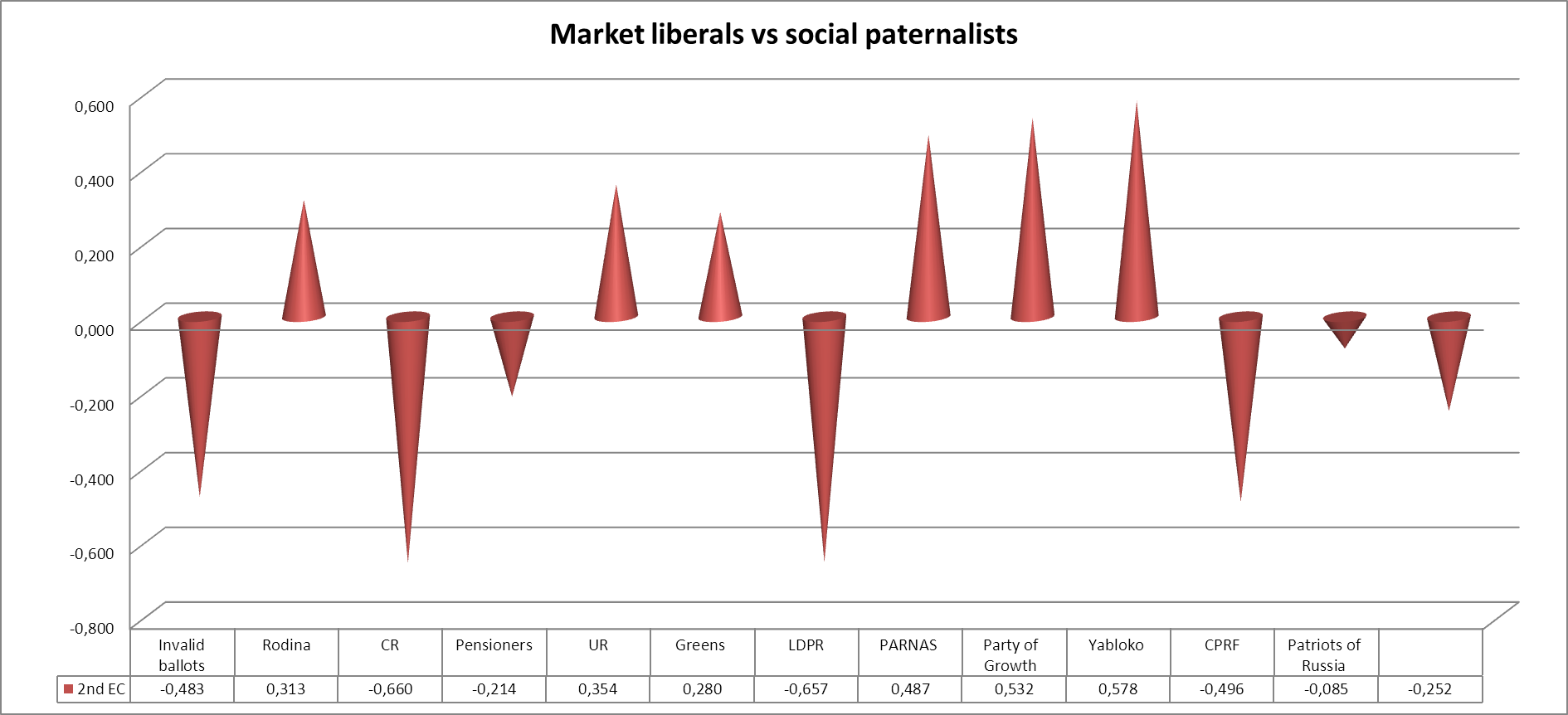
Figure 1. The configuration of the second electoral cleavage during the 2016 Russian legislative election. Disambiguation: Rodina – “Rodina” Party; CR – Communists of Russia; RPPSJ – Russian Party of Pensioners for Social Justice; UR – United Russia; REPG – Russian Ecological Party “The Greens”; CP – Civic Platform; LDPR – Liberal Democratic Party of Russia; PARNAS – People's Freedom Party; PG – Party of Growth (before 2016: RC – Right Cause); CivPo – Civilian Power; Yabloko – Russian United Democratic Party “Yabloko”; CPRF – Communist Party of the Russian Federation; PR – Patriots of Russia; AJR – A Just Russia.
It turns out that the voter's choice does not always demonstrate the power balance dynamics in political space. This, naturally, comes as no surprise. While focusing on the difference in positions, factor analysis does not reveal cleavages in political space per se but rather dimensions and political factions. In our case factor analysis discovered the "party of power", liberals and social paternalists, all of whom have quite a complicated relationship. Point is, even those directly involved in political power struggle – parties above all – seldom realize the complexity of this relationship. That being the case, it is no surprise that regular voters are unable (and unwilling) to untangle this cobweb, and luckily this is none of their concern.
One key feature of political mass consciousness should be considered in particular. All deviations aside, political parties (much like the political establishment as a whole) have quite a comprehensive understanding of the structure of political space. Mass consciousness on the other hand lives by Plato's allegory of the cave where people sit with their backs turned to the entrance and judge the outside world by the shadows on the walls. Among voters, there are people well versed in politics, however most of them only choose whatever pieces resonate with them personally without taking heed of the entire information flow.
For that reason the political dimensions determined through factor analysis may or may not coincide with political cleavages in electoral space. Lack of coincidence points at a highly fragmented electoral space, scant knowledge of actual political landscape in voters, etc.
It is necessary to consider this fragmented nature while determining the political undertone of electoral cleavages. Although there is obviously no need to resort to singular issues, we can safely compare their positions in more generalized issues domains.
For that purpose, we conducted a factor analysis of party lines concerning the issues pertaining three separate domains: home policy issues, socioeconomic issues and systemic issues (foreign policy + ideology). The results were as follows.
Three cleavages emerged for home policy issues (Table 2):
1) between United Russia and the rest of the parties; the main points of disagreement are Russian Academy of Sciences (RAS) reform, municipal reform, extending the powers of parliament, removing the municipal filter;
2) between liberals (Yabloko, PARNAS) and loyalists (United Russia, The Greens, Party of Pensioners, Rodina): attitude to Putin, "Yarovaya Law," "foreign agent" law, defining the current political regime as authoritarian;
3) between social patriots (A Just Russia, Patriots of Russia, CPRF) and loyalists (Party of Pensioners, The Greens, Party of Growth): switching to voluntary enlistment (professional army), defining the current political regime as authoritarian, "Yarovaya Law."
Table 2. Cleavage factors by domestic agenda during the 2016 elections
| Variable | Factor Loadings (Unrotated) (Spreadsheet1) | ||
| Extraction: Principal components | |||
| (* >.700000) | |||
| Factor 1 | Factor 2 | Factor 3 | |
| Rodina | -0.599 | -0.665 | -0.004 |
| Communists of Russia | -0.704 * | -0.492 | -0.194 |
| Russian Party of Pensioners for Social Justice | -0.183 | -0.766 * | 0.536 |
| United Russia | 0.658 | -0.700 | -0.203 |
| Russian Ecological Party “The Greens” | -0.352 | -0.813 * | 0.420 |
| LDPR | -0.548 | 0.089 | 0.208 |
| PARNAS | -0.668 | 0.704 * | 0.189 |
| Party of Growth | -0.845 * | 0.047 | 0.421 |
| Yabloko | -0.697 | 0.674 | 0.191 |
| CPRF | -0.847 * | 0.248 | -0.361 |
| Patriots of Russia | -0.799 * | -0.386 | -0.337 |
| A Just Russia | -0.710 * | -0.310 | -0.557 |
| Expl.Var | 5.254 | 3.689 | 1.388 |
| Prp.Totl | 43.78% | 30.74% | 11.57% |
Socioeconomic issues displayed three cleavages as well (Table 3):
1) between United Russia and systemic opposition (CPRF, LDPR, A Just Russia, Rodina, Patriots of Russia, Communists of Russia): raising the retirement age, views on private ownership and government intervention in the economy, government activities;
2) between communists (CPRF, Communists of Russia) and liberals (Yabloko, PARNAS, Party of Growth): views on capitalism, private ownership, nationalization, contribution pension scheme, government intervention in the economy, "optimizing" healthcare and education systems;
3) between loyalists (United Russia, Party of Pensioners, The Greens) and marginalized ideologized opposition (PARNAS, Communists of Russia, Yabloko): views on building renovation fee, contribution pension scheme, pension underindexation, increasing military expenditure.
Table 3. Subdivisions of socioeconomic issue domain in the 2016 election
| Variable | Factor Loadings (Unrotated) (Spreadsheet1) | ||
| Extraction: Principal components | |||
| (* >.700000) | |||
| Factor 1 | Factor 2 | Factor 3 | |
| Rodina | -0.767 * | 0.234 | 0.213 |
| Communists of Russia | -0.872 * | -0.297 | -0.220 |
| Russian Party of Pensioners for Social Justice | -0.412 | 0.266 | 0.570 |
| United Russia | 0.411 | 0.102 | 0.728 * |
| Russian Ecological Party “The Greens” | -0.091 | 0.580 | 0.466 |
| LDPR | -0.841 * | 0.178 | 0.108 |
| PARNAS | 0.019 | 0.917 * | -0.307 |
| Party of Growth | -0.181 | 0.837 * | -0.168 |
| Yabloko | -0.125 | 0.895 * | -0.256 |
| CPRF | -0.917 * | -0.288 | -0.113 |
| Patriots of Russia | -0.928 * | -0.089 | 0.185 |
| A Just Russia | -0.924 * | -0.098 | -0.056 |
| Expl.Var | 5.008 | 3.036 | 1.417 |
| Prp.Totl | 41.73% | 25.30% | 11.81% |
The third area of concern manifested as a clear distinction of foreign policy ("imperialists"–"anti-imperialists") and world views (progressivists–traditionalists; views on capitalism, Russian exceptionalism, Eurasian integration, switching to professional army) (Table 4).
Table 4. Subdivisions of international and worldview issue domain in the 2016 election
| Factor Loadings (Unrotated) (Spreadsheet2) | ||
| Variable | Extraction: Principal components | |
| (* >.700000) | ||
| Factor | Factor | |
| 1 | 2 | |
| Rodina | -0.962 * | -0.138 |
| Communists of Russia | -0.819 * | -0.086 |
| Russian Party of Pensioners for Social Justice | -0.590 | 0.414 |
| United Russia | -0.794 * | 0.275 |
| Russian Ecological Party “The Greens” | -0.728 * | 0.366 |
| LDPR | -0.879 * | -0.004 |
| PARNAS | 0.952 * | 0.230 |
| Party of Growth | -0.366 | 0.763 * |
| Yabloko | 0.936 * | 0.233 |
| CPRF | -0.947 * | -0.269 |
| Patriots of Russia | -0.941 * | -0.062 |
| A Just Russia | -0.950 * | -0.053 |
| Expl.Var | 8.476 | 1.176 |
| Prp.Totl | 70.63% | 9.80% |
If we compare factor loadings for these eight sub-dimensions (Table 5) we will see that the first authoritarian-democratic ("government vs opposition") correlates closely with the first and third socioeconomic ones ("government vs systemic opposition" and "government vs liberal opposition"); the second authoritarian-democratic (liberals vs loyalists) correlates with the third socioeconomic and the "imperialistic–anti-imperialistic" version of systemic sub-dimension; the third authoritarian-democratic (social patriots vs liberals) correlates with the second socioeconomic (communists vs liberals) and second systemic (statists vs liberals). Second systemic also shares a close connection with second socioeconomic and third authoritarian-democratic sub-dimensions, etc. It is thus clear that the three initially indicated dimensions are hybrids by nature, meaning they contain elements from all kinds of areas and the labels attached to them (authoritarian-democratic, socioeconomic, systemic) are in fact purely theoretical. They rather indicate political factions than political cleavages.
Table 5. Correlation of political space sub-dimensions relative to one another
| Correlations (Spreadsheet1) | ||||||||
| Variable | * correlations are significant at p < .05000 | |||||||
| N=14 (Casewise deletion of missing data) | ||||||||
| AD-GO | AD-LL | AD-SPL | SE-ASO | SE-CL | SE-ALO | Syst-IA | Syst-SL | |
| AD – government vs opposition | 1 | -0.305 | 0.059 | 0.782 * | 0.175 | 0.612 * | 0.098 | 0.222 |
| p= --- | p=.290 | p=.840 | p=.001 | p=.550 | p=.020 | p=.740 | p=.445 | |
| AD – liberals vs loyalists | -0.305 | 1 | 0.006 | -0.163 | 0.212 | -0.850 * | 0.676 * | -0.046 |
| p=.290 | p= --- | p=.984 | p=.579 | p=.468 | p=.000 | p=.008 | p=.877 | |
| AD – social patriots vs liberals | 0.059 | 0.006 | 1 | 0.418 | 0.779 * | 0.06 | 0.442 | 0.740 * |
| p=.840 | p=.984 | p= --- | p=.137 | p=.001 | p=.840 | p=.113 | p=.002 | |
| SE – government vs systemic opposition | 0.782 * | -0.163 | 0.418 | 1 | 0.645 * | 0.358 | 0.429 | 0.667 * |
| p=.001 | p=.579 | p=.137 | p= --- | p=.013 | p=.209 | p=.126 | p=.009 | |
| SE – communists vs liberals | 0.175 | 0.212 | 0.779 * | 0.645 * | 1 | -0.107 | 0.679 * | 0.863 * |
| p=.550 | p=.468 | p=.001 | p=.013 | p= --- | p=.716 | p=.008 | p=.000 | |
| SE – government vs liberal opposition | 0.612 * | -0.850 * | 0.060 | 0.358 | -0.107 | 1 | -0.523 | 0.074 |
| p=.020 | p=.000 | p=.840 | p=.209 | p=.716 | p= --- | p=.055 | p=.802 | |
| Syst – “imperialists” vs “anti-imperialists” | 0.098 | 0.676 * | 0.442 | 0.429 | 0.679 * | -0.523 | 1 | 0.423 |
| p=.740 | p=.008 | p=.113 | p=.126 | p=.008 | p=.055 | p= --- | p=.132 | |
| Syst – statists vs liberals | 0.222 | -0.046 | 0.740 * | 0.667 * | 0.863 * | 0.0739 | 0.4229 | 1 |
| p=.445 | p=.877 | p=.002 | p=.009 | p=.000 | p=.802 | p=.132 | p= --- | |
As for correlation between factor loadings of electoral cleavages and sub-dimensions mentioned above (Table 6), it seems our instincts were right: the second electoral cleavage was indeed closely correlated with the communist and anti-communist factions competition in socioeconomic field, since it exhibits the highest correlation module and the lowest p-level. At the same time, factor loadings of this EC correlate closely with another form of socioeconomic dimension (United Russia vs systemic opposition) as well with both forms of systemic dimension (foreign policy and world views).
Table 6. Correlation between electoral cleavages and political sub-dimensions during the 2016 legislative election
| Correlations (Spreadsheet2) | ||||||||
| Variable | * correlations are significant at p < .05000 | |||||||
| N=12 (Casewise deletion of missing data) | ||||||||
| AD-GO | AD-LL | AD-SPL | SE-ASO | SE-CL | SE-ALO | Syst-IA | Syst-SL | |
| Electoral cleavage-1 | -0.618 * | 0.312 | 0.573 | -0.182 | 0.496 | -0.395 | 0.376 | 0.184 |
| p=.032 | p=.324 | p=.051 | p=.571 | p=.101 | p=.204 | p=.228 | p=.567 | |
| Electoral cleavage-2 | 0.183 | 0.191 | 0.381 | 0.753 * | 0.806 * | 0.033 | 0.599 * | 0.605 * |
| p=.569 | p=.553 | p=.222 | p=.005 | p=.002 | p=.920 | p=.039 | p=.037 | |
| Electoral cleavage-3 | -0.145 | -0.068 | -0.093 | -0.167 | -0.163 | 0.081 | -0.122 | -0.226 |
| p=.654 | p=.833 | p=.774 | p=.604 | p=.612 | p=.802 | p=.705 | p=.480 | |
However, after building the regression model that uses electoral cleavages as dependent variables and the revealed additional dimensions (Table 7) as independent variables we discovered that the nature of the second EC is completely defined by the communist-liberal sub-dimension of the socioeconomic political dimension. If we remove the SE-2 independent variable from the model, the rest of the remaining sub-dimensions will manifest themselves one by one. They will also display a significant correlation with the second electoral cleavage, but their determination coefficients will be significantly lower and there will be no cumulative effect whatsoever. Besides, the squared multiple regression (coefficient of determination) in this model gives a significant boost to the corresponding parameter if the "main" political dimensions are used as independent variables.
Table 7. Multiple regression (OSL model) of the connection between electoral cleavages and political dimensions and sub-dimensions
| EC-1 | EC-2 | |||
| Model 1 | Model 2 | Model 1 | Model 2 | |
| Determination coefficients (R2) | 0.465 | 0.788 | 0.464 | 0.65 |
| Beta-coefficients (standard error) | ||||
| Systemic issue dimension | - | - | 0.681 (0.231) | - |
| Authoritarian-democratic issue dimension | -0.682 (0.231) | - | - | - |
| Socioeconomic issue dimension | - | - | - | - |
| AD-1 (government–opposition) | - | -0.681 (0.154) | - | - |
| AD-2 (loyalists–liberals) | - | - | - | - |
| AD-3 (social-paternalists–liberals) | - | 0.641 (0.154) | - | - |
| SE-1 (authority–systemic opposition) | - | - | - | |
| SE-2 (communists–liberals) | - | - | - | 0.806 (0.187) |
| SE (loyalists–ideologized opposition) | - | - | - | - |
| Systemic 1 ("imperialists"–"anti-imperialists") | - | - | - | - |
| Systemic 2 (traditionalists–progressivists) | - | - | - | - |
The results are even more impressive after applying this model to the first electoral cleavage. Two authoritarian-democratic political dimension forms at once turned out to be predictors: "government vs opposition" and "social paternalists vs liberals." This seems logical, especially since the "main" version of the authoritarian-democratic political dimension has to do with the competition between the government and liberals, and the former did not do very well in the 2016 elections. Moreover, the coefficient of determination in this model is significantly higher than the corresponding parameter in the model using "main" political dimensions.
For future reference, we therefore offer not to limit the comparison of factor loadings of parties in electoral space to the three "main" dimensions, but also utilize the factor loadings within the additional eight sub-dimensions. This will allow to further improve the method used to calculate the politicization coefficient of an electoral cleavage. First, we used the coefficient of correlation between political and electoral cleavages whose module was multiplied by effective range coefficient of an EC. Squared multiple regression (coefficient of determination) is much more appropriate for this formula (especially since this allows to standardize the calculation of politicization and socialization coefficients), but before there was not many political cleavages to choose from, which hindered its use (although in truth this was not much of a hindrance, since two independent variables are enough for multiple regression). Now this advantage of the regression model over the correlation model is obvious while calculating electoral cleavage politicization coefficient.
We therefore propose to make future calculations of the electoral cleavage politicization coefficient as follows: \(Pc = Ec R^2\), where \(R^2\) is the coefficient of determination for the connection between the EC and a set of political dimensions. The calculation should be split in two models, where the first one requires using the three "main" dimensions as independent variables while the second one requires additional sub-dimensions to be used. Whichever squared multiple regression is higher (and it has been proved that results vary a lot), that one will be used to calculate the electoral cleavage politicization coefficient. It has been defined empirically that putting main and additional dimensions into a single model makes for limited results than splitting the calculations into two models.
The new instruments are not the only novelty in this method, however. The previous method was based on the premise that political cleavages were identical in structure for every federal subject. Is such a theory justified, however? The question is whether this is the same structure as in Chechnya, where United Russia won by a 99.5% landslide; in Kabardino-Balkaria, where the competition between the "party of power" and communists was famously fierce and in Tomsk and Moscow Oblasts for instance, where even such party as Right Cause was able to gain 1% of votes.
Besides, the number of participants who received a more or less significant amount of votes affects the number of political cleavages revealed via factor analysis. For example, Tomsk and Moscow Oblasts presented three such cleavages each. Kabardino-Balkaria presented one while Chechnya did not present any. It is therefore appropriate to split federal subjects into groups according to the number and structure of the parties that received >1% vote count there, then use factor analysis on these participants only and reveal the actual structure of cleavages in the corresponding federal subjects. It is their factor loadings that should be compared with their own factor loadings in electoral space once these factor loadings has been recalculated after the participants with less than 1% votes were filtered out.
This will be the first stage of the research. The second stage implies calculating maximum and effective range coefficients as well as politicization and socialization coefficients of electoral cleavages using the formulas described before (with the above-mentioned adjusted politicization formula).
The third stage implies sorting regions based on several criteria: number of electoral cleavages, EC structure, maximum and effective range, socialization coefficient, authoritarian-democratic cleavage balance ratio (the corresponding coefficient calculated as follows: \(Rc= Mс_{min} / Mс_{max}\), where \(Mс_{min}\) is the weaker side range, and \(Mс_{max}\) stronger side range). Underlying the structure of the electoral cleavages is their number in the region, maximum and effective range coefficients as well as politicization and socialization coefficients of the ECs.
The fourth and final stage of the research implies a cluster analysis of beta-coefficients of main and additional political dimensions connected with electoral cleavages within the framework of corresponding regression models (only the cases with a ≤10% margin of error are taken into account). Other criteria are considered as well, namely politicization and socialization coefficients of electoral cleavages in the region and the number of votes for United Russia.
The 2011 legislative election and cleavage structure in the regions
As can be seen in Table 8, most federal subjects had their structure of political cleavages determined by five of six parties that gained more than 1% of votes. The first group included 33 federal subjects, while the second included 35. In the first case it comes to four parliamentary parties and Yabloko while in the second case it is the previous five and the Patriots of Russia (only Sverdlovsk Oblast presented a "Five + Right Cause" combination).
Table 8. The structure of political dimensions in the regions during the 2011 legislative election
| No. of parties with ≥ 1 % votes | No. of cleavages | No. of regions | Parties | Regions |
| 1 | 0 | 1 | United Russia | Chechen Republic |
| 2 | 1 | 4 | United Russia, CPRF | Republics: Dagestan, Kabardino-Balkaria, Karachay-Cherkessia, Mordovia |
| 4 | 1 | 5 | United Russia, CPRF, A Just Russia, LDPR | Republics: Bashkortostan, Kalmykia, North Ossetia, Tatarstan, Tyva; Astrakhan Oblast |
| 4 | 1 | 1 | United Russia, CPRF, A Just Russia, Right Cause | Republic of Ingushetia |
| 5 | 2 | 33 | United Russia, CPRF, A Just Russia, LDPR, Yabloko | Republics: Adygea, Altai, Mari El, Buryatia, Karelia, Yakutia; Krais: Altai, Zabaykalsky, Krasnodar, Krasnoyarsk, Primorsky, Stavropol; Oblasts: Belgorod, Bryansk, Voronezh, Kemerovo, Kurgan, Lipetsk, Nizhny Novgorod, Novgorod, Oryol, Penza, Pskov, Rostov, Saratov, Tambov, Tula, Tyumen, Ulyanovsk, Chelyabinsk; Jewish Autonomous Oblast; Chukotka and Yamalo-Nenets Autonomous Okrugs |
| 6 | 2 | 1 | United Russia, CPRF, A Just Russia, LDPR, Yabloko, Right Cause (Party of Growth) | Sverdlovsk Oblast |
| 6 | 3 | 35 | United Russia, CPRF, A Just Russia, LDPR, Yabloko, Patriots of Russia | Republics: Komi, Udmurtia, Khakassia, Chuvashia; Krais: Kamchatka, Perm, Khabarovsk; Oblasts: Amur, Arkhangelsk with Nenets AO, Vladimir, Volgograd, Vologda, Ivanovo, Irkutsk, Kaliningrad, Kaluga, Kirov, Kostroma, Kursk, Leningrad, Magadan, Murmansk, Novosibirsk, Omsk, Orenburg, Ryazan, Samara, Sakhalin, Smolensk, Tver, Yaroslavl; Moscow, Saint-Petersburg, Khanty-Mansi Autonomous Okrug |
| 7 | 3 | 2 | United Russia, CPRF, A Just Russia, LDPR, Yabloko, Patriots of Russia, Right Cause | Moscow and Tomsk Oblasts |
The "four parliamentary parties + Yabloko" combination produced a two-dimensional political space. Based on the issues with the highest modular factor scores, the first factor (Figure 2) was a combination of authoritarian-democratic and systemic dimensions (Table 9) while the second factor (Figure 3) was mostly socioeconomic (Table 10).
Figure 2. First political dimension in the regions displaying the "4 parliamentary parties + Yabloko" combination during the 2011 legislative election.
Table 9. Issues with highest factor scores during the 2011 legislative election in the regions displaying the "4 parliamentary parties + Yabloko" combination upon first dimension
| Issue | AJR | LDPR | CPRF | Yabloko | UR | Factor scores |
| Degree of opposition (self-evaluation) | 5 | 5 | 5 | 5 | -5 | -1.301 |
| The government violating election law | 5 | 5 | 5 | 5 | -5 | -1.301 |
| Ratifying Article 20 of the United Nations Convention Against Corruption | 5 | 5 | 5 | 5 | -2 | -1.104 |
| Free healthcare and education | 5 | 5 | 5 | 3 | -3 | -1.078 |
| Establishing state monopoly on alcohol | 5 | 5 | 5 | 0 | -5 | -1.073 |
| Reinstating proper electoral procedure, expanding political competition | 5 | 3 | 5 | 5 | -4 | -1.056 |
| Using reserve funds for government spending | 5 | 5 | 5 | -1 | -5 | -1.027 |
| … | … | … | … | … | … | … |
| Attitude towards the Soviet past | -3 | -4 | 5 | -5 | -3 | 1.08 |
| Removing Lenin's body from the Mausoleum | -3 | 5 | -5 | 5 | 3 | 1.17 |
| Bringing back single-member district elections | 2 | -5 | -5 | 0 | 0 | 1.48 |
| Legalizing firearms for civilian use | -5 | 3 | -5 | -5 | -5 | 1.527 |
| Joining the WTO | 0 | -5 | -4 | 5 | 5 | 1.731 |
| Raising the retirement age | -5 | -5 | -5 | -5 | -3 | 2.375 |
| Attitude to Putin | -3 | -3 | -5 | -4 | 5 | 2.428 |

Figure 3. Second political dimension in the regions displaying the "4 parliamentary parties + Yabloko" combination during the 2011 legislative election.
Table 10. Issues with highest factor scores during the 2011 legislative election in the regions displaying the "4 parliamentary parties + Yabloko" combination upon second dimension
| Issue | AJR | LDPR | CPRF | Yabl | UR | Factor scores |
| Joining the WTO | 0 | -5 | -4 | 5 | 5 | -2.184 |
| Removing Lenin's body from the Mausoleum | -3 | 5 | -5 | 5 | 3 | -2.039 |
| Prohibiting flashing lights on state officials' vehicles | 5 | 4 | -3 | 5 | -4 | -1.441 |
| Nullifying resident registration | 5 | 3 | -5 | 3 | -3 | -1.399 |
| Replacing compulsory military service with voluntary enlistment | -5 | 5 | -5 | 5 | -5 | -1.119 |
| Extending the powers of parliament | 5 | 5 | 5 | 5 | 0 | -1.014 |
| Closing down offshore accounts | 5 | 5 | 5 | 5 | 0 | -1.014 |
| … | … | … | … | … | … | … |
| Nationalization | 3 | 0 | 4 | -5 | -3 | 1.071 |
| Switching back from contribution pension scheme to distribution pension scheme | 5 | -1 | 4 | -5 | -4 | 1.096 |
| Introducing graduated income tax and wealth tax | 5 | 5 | 5 | -5 | -4 | 1.15 |
| Abolishing private ownership of land | -3 | -3 | 4 | -4 | -4 | 1.291 |
| Reintroducing capital punishment | -5 | 5 | 5 | -5 | -2 | 1.381 |
| Restoring the “Ethnic Origin” field in passports | -1 | -2 | 4 | -5 | -5 | 1.473 |
| Decriminalizing Article 282 of the Criminal Code | 0 | 5 | 5 | -5 | -5 | 1.474 |
| Attitude towards the Soviet past | -3 | -4 | 5 | -5 | -3 | 1.477 |
Factor analysis of separate issue domains revealed two cleavages in socioeconomic domain ("marketeers vs protectionists" and "communists vs anti-communists"), two cleavages in home policy ("government vs opposition" and "conservatives vs liberals") and two cleavages in systemic dimension ("civil activists vs statists" and "communists vs anti-communists").
The "four parliamentary parties + Yabloko + Right Cause" combination also produced a two-dimensional political structure but with a hierarchy that was in turn produced by the five-party combination. In this case, the first place was occupied by the socioeconomic dimension (Figure 4) while the second was occupied by a hybrid of authoritarian-democratic and systemic dimensions (Figure 5).
Figure 4. First political dimension in the regions displaying the "4 parliamentary parties + Yabloko + Right Cause" combination during the 2011 legislative election.
Figure 5. Second political dimension in the regions displaying the "4 parliamentary parties + Yabloko + Right Cause" combination during the 2011 legislative election.
For issue domains level, the difference with five-party combination was in one more sub-dimension ("universalists vs federalists") that joined the existing two (authoritarian-democratic in nature). The systemic dimension saw the "civil activists vs statists" and "communists vs anti-communists" cleavages exchange their positions.
The "four parliamentary parties + Yabloko + Patriots of Russia" combination produced the same three-dimensional structure as the full (seven-party) combination: socioeconomic dimension was in the first place, systemic was in the second while authoritarian-democratic was in the third [16].
As for issue domains level, factor analysis revealed sub-dimensions identical to the previous case, except the systemic dimension saw the "civil activists vs statists" polarity reclaim the first place.
The third most prevalent combination (although far behind the first two) was the four-party one, manifesting in two variations: 1) four parliamentary parties (Bashkortostan, Kalmykia, North Ossetia, Tatarstan, Tyva and Arkhangelsk Oblast); 2) "United Russia + CPRF + A Just Russia + Right Cause" (Ingushetia). In the first case, the political cleavage structure boiled down to competition between United Russia and parliamentary opposition while in the second case there was competition between "party of power" and Right Cause on the one hand and CPRF and A Just Russia on the other (Figure 6). However, both cases saw three dimensions join into one: United Russia (along with Right Cause in the second case) simultaneously competed against parliamentary opposition parties as both the government and the marketeer against opposition and anti-marketeers respectively.
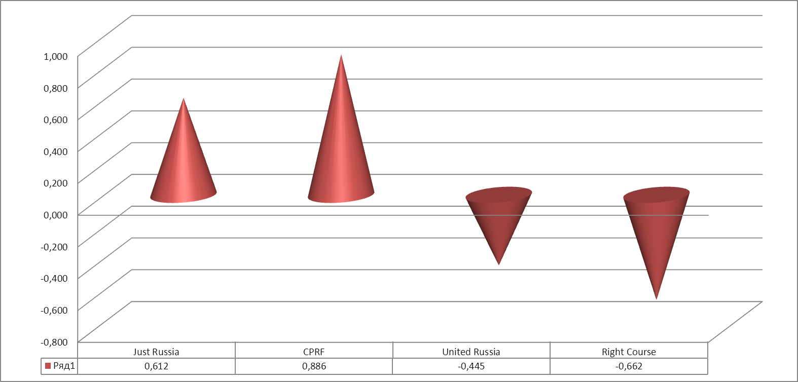
Figure 6. Political cleavage in Ingushetia during the 2011 legislative election.
As for the issue domains analysis level, it presented only one socioeconomic sub-dimension ("marketeers vs protectionists"), two home policy sub-dimensions ("government vs opposition" and "conservatives vs liberals") and two systemic sub-dimensions ("social activists vs statists" and "communists vs anti-communists").
Four regions (Dagestan, Kabardino-Balkaria, Karachay-Cherkessia and Mordovia) presented the "two-party system": CPRF was United Russia's only competitor, albeit falling behind in vote count (Kabardino-Balkaria "spearheaded" this group of regions with a communist vote count of 18% against ~9% in Karachay-Cherkessia, ~8% in Dagestan and ~5% in Mordovia). It is clear that in the "party of power vs CPRF" standoff all three dimensions joined once again.
Only two federal subjects (Tomsk and Moscow Oblasts) saw all seven (at the time) registered political parties hop over the 1% barrier. Naturally, the cleavage structure here was three-dimensional while issue domains analysis revealed sets of sub-dimensions that were almost identical to the "four parliamentary parties + Yabloko + Patriots of Russia" combination, except for in the home policy dimension the "conservatives vs liberals" cleavage rose to the first place and the "government vs opposition" cleavage moved down to the second and transformed into "government vs liberals."
Finally, the Chechen Republic was a standalone case since with 99.5% of votes for United Russia, there was no room for cleavages whatsoever.
Now let us move on to electoral cleavages. Table 11 displays their values in regions while only taking parties with >1% vote count into account. The data is filtered by the number of electoral cleavages, and as we can see this number never went over three. Besides, the group of regions with three ECs is the least numerous and was comprised from 11 regions only, including Saint Petersburg and Moscow Oblast. These regions were characterized by low voter turnout, low United Russia vote count, moderate maximum range coefficients and sizeable coefficients of effective range, socialization and politicization on the main cleavage. The only exceptions were Ivanovo, Kirov and Kostroma Oblasts where the margin of error for connection between electoral and political cleavages went over 10% so the politicization coefficient amounted to zero. The second and third electoral cleavages revealed much smaller maximum and effective range coefficients with socialization and politicization coefficients going even lower.
Table 11. Regions grouped by the number of electoral cleavages during the 2011 elections, a) No cleavages
| Region | Turnout | UR results (%) | No. of parties with more than 1% of votes |
| Chechen Republic | 99.45 | 99.48 | 1 |
b) One cleavage
| Region | Turnout | UR results (%) | No. of parties with more than 1% of votes | No. of electoral cleavages (dimensions) | EC-1 | ||||
| Max. range coef. | Eff. range coef. | Politicization coef. | Socialization coef. | ||||||
| 1 | Republic of Dagestan | 89.37 | 91.46 | 2 | 1 | 99.13 | 15.78 | - | 0 |
| 2 | Kabardino-Balkar Republic | 98.27 | 81.91 | 2 | 1 | 99.49 | 35.24 | - | 0 |
| 3 | Karachay-Cherkess Republic | 93.14 | 89.84 | 2 | 1 | 98.54 | 17.62 | - | 6 |
| 4 | Republic of Mordovia | 96.06 | 91.62 | 2 | 1 | 96.09 | 9.07 | - | 2.55 |
| 5 | Republic of Bashkortostan | 83.5 | 70.32 | 4 | 1 | 94.09 | 50.25 | 47.68 | 16.88 |
| 6 | Republic of Kamlykia | 67.95 | 66.1 | 4 | 1 | 93.28 | 55.18 | 54.99 | 30.86 |
| 7 | Komi Republic | 71.78 | 58.81 | 6 | 3 | 85.7 | 57.05 | 46.66 | 0 |
| 8 | Mari El Republic | 75.7 | 52.24 | 5 | 2 | 93.54 | 83.09 | 76.48 | 43.51 |
| 9 | Republic of Tatarstan | 89.28 | 76.82 | 4 | 1 | 96.07 | 38.79 | 38.73 | 29.84 |
| 10 | Tyva Republic | 89.07 | 85.29 | 4 | 1 | 94.02 | 21.21 | 21.21 | 6.67 |
| 11 | Belgorod Oblast | 81.55 | 51.16 | 5 | 2 | 92.26 | 83.49 | 77.31 | 51.61 |
| 12 | Voronezh Oblast | 70.4 | 48.07 | 5 | 2 | 91.79 | 87.9 | 78.03 | 44.34 |
| 13 | Lipetsk Oblast | 60.12 | 40.09 | 5 | 2 | 82.34 | 78.82 | 74.48 | 64.92 |
| 14 | Omsk Oblast | 63.68 | 38.04 | 6 | 3 | 86.93 | 75.16 | 65.54 | 61.91 |
| 15 | Penza Oblast | 69.62 | 56.3 | 5 | 2 | 94.02 | 76.59 | 70.23 | 51.83 |
| 16 | Saratov Oblast | 70.36 | 64.89 | 5 | 2 | 93.47 | 57.77 | 53.15 | 14.95 |
| 17 | Tyumen Oblast | 83.53 | 62.21 | 5 | 2 | 96.29 | 68.37 | 62.85 | 46.27 |
| 18 | Ulyanovsk Oblast | 66.98 | 43.56 | 5 | 2 | 90.95 | 86.77 | 80.75 | 66.59 |
The table is not fully displayed Show table
c) Two cleavages (beginning)
| Region | Turnout | UR results (%) | No. of parties with more than 1% of votes | No. of PDs | EC-1 | EC-2 | |||||||
| Mc | Ec | Pc | Sc | Mc | Ec | Pc | Sc | ||||||
| 1 | Republic of Adygea | 70.96 | 61 | 5 | 2 | 88.53 | 55.55 | 53.29 | 0 | 21.75 | 19 | 0 | 0 |
| 2 | Altai Republic | 65.18 | 53.33 | 5 | 2 | 90.4 | 74.97 | 64.31 | 52.92 | 11.48 | 9.38 | 0 | 0 |
| 3 | Republic of Buryatia | 58.67 | 49.02 | 5 | 2 | 79.41 | 62.56 | 56.26 | 46.93 | 35.61 | 31.78 | 0 | 12.33 |
| 4 | Republic of Ingushetia | 86.66 | 90.96 | 4 | 1 | 95.46 | 10.41 | 0 | 0 | 5.84 | 0.89 | 0 | 0 |
| 5 | Republic of Karelia | 49.2 | 32.26 | 5 | 2 | 61.36 | 53.07 | 50.79* | 20.5 | 45.34 | 43.43 | 0 | 12.17 |
| 6 | Republic of North Ossetia | 67.06 | 67.9 | 4 | 1 | 90.19 | 46.48 | 46.12 | 0 | 17.49 | 11.14 | 0 | 4.56 |
| 7 | Yakutia Republic | 83.23 | 49.16 | 5 | 2 | 71.39 | 42.65 | 0 | 5.93 | 46.46 | 40.2 | 0 | |
| 8 | Udmurt Republic | 60.49 | 45.09 | 6 | 3 | 79.28 | 70.43 | 53.9 | 0 | 9.94 | 8.99 | 0 | 0 |
| 9 | Republic of Khakassia | 59.47 | 40.13 | 6 | 3 | 77.78 | 76.75 | 73.18 | 61.15 | 32.52 | 28.64 | 3.41 | 0 |
| 10 | Chuvash Republic | 64.55 | 43.42 | 6 | 3 | 86.35 | 85.76 | 81.05 | 70.87 | 7.38 | 5.24 | 0 | 0 |
| 11 | Zabaykalsky Krai | 55.27 | 43.28 | 5 | 2 | 76.7 | 68.73 | 62.04 | 44.8 | 26.01 | 22.69 | 0 | 14.49 |
| 12 | Kamchatka Krai | 61.71 | 45.25 | 6 | 3 | 73.26 | 62.27 | 38.51 | 50.58 | 36.29 | 31.93 | 11.7 | 10.84 |
| 13 | Krasnodar Krai | 72.33 | 56.18 | 5 | 2 | 87.68 | 63.45 | 59.16 | 0 | 14.4 | 11.72 | 0 | 4.18 |
| 14 | Primorsky Krai | 49.89 | 32.99 | 5 | 2 | 69.64 | 62.56 | 59.76 | 44.08 | 33.69 | 30.99 | 0 | 0 |
| 15 | Stavropol Krai | 49.68 | 49.11 | 5 | 2 | 82.79 | 68.56 | 68.16 | 18.04 | 18.73 | 17.41 | 36.76 | 9.17 |
| 16 | Khabarovsk Krai | 55.4 | 38.14 | 6 | 3 | 71.03 | 69.68 | 69.67 | 56.7 | 39.67 | 36.83 | 19.89 | 21.97 |
| 17 | Amur Oblast | 56.67 | 43.54 | 6 | 3 | 83.14 | 81.61 | 70.16 | 58.18 | 23.56 | 22.78 | 0 | 0 |
| 18 | Arkhangelsk Oblast + Nenets AO | 51.1 | 36.01 | 6 | 3 | 60.21 | 56.22 | 51.78* | 47.31 | 48.83 | 41.34 | 10.67 | 28.91 |
The table is not fully displayed Show table
(end)
| Region | Turnout | UR results (%) | No. of parties with more than 1% of votes | No. of PDs | EC-1 | EC-2 | |||||||
| Mc | Ec | Pc | Sc | Mc | Ec | Pc | Sc | ||||||
| 27 | Kurgan Oblast | 59.74 | 44.41 | 5 | 2 | 79.07 | 71.93 | 68.45 | 29.84 | 29.58 | 28.93 | 0 | 16.38 |
| 28 | Kursk Oblast | 58.48 | 45.72 | 6 | 3 | 84.82 | 79.65 | 62.98 | 57.16 | 12.32 | 9.54 | 0 | 0 |
| 29 | Magadan Oblast | 54.4 | 41.04 | 6 | 3 | 89.07 | 80.59 | 78.68 | 47.35 | 28.04 | 27.23 | 0 | 0 |
| 30 | Murmansk Oblast | 52.88 | 32.02 | 6 | 3 | 73.57 | 69.82 | 43.12* | 64.58 | 34.4 | 31.37 | 0 | 22.45 |
| 31 | Nizhny Novgorod Oblast | 63.22 | 43.91 | 5 | 2 | 79.32 | 73.9 | 70.41 | 30.63 | 29.29 | 28.16 | 0 | 7.51 |
| 32 | Novgorod Oblast | 58.97 | 34.58 | 5 | 2 | 75.08 | 66.62 | 60.85 | 46.21 | 26.41 | 24.77 | 23.18 | 0 |
| 33 | Novosibirsk Oblast | 58.96 | 33.84 | 6 | 3 | 75.12 | 74.61 | 49.46 | 67.22 | 32.91 | 27.02 | 0 | 5.14 |
| 34 | Orenburg Oblast | 53.42 | 34.96 | 6 | 3 | 65.7 | 65.57 | 64.02* | 49.41 | 35.51 | 26.54 | 0 | 6.04 |
| 35 | Oryol Oblast | 67.39 | 38.99 | 5 | 2 | 88.24 | 76.75 | 72.13 | 46.47 | 13.54 | 10.1281 | 0 | 0 |
| 36 | Pskov Oblast | 54.51 | 36.65 | 5 | 2 | 76.9 | 72.83 | 69.37 | 39.1 | 24.38 | 23.7 | 0 | 7.23 |
| 37 | Rostov Oblast | 60.63 | 50.082 | 5 | 2 | 89.48 | 79.02 | 72.91 | 26.36 | 7.35 | 4.44 | 0 | 0.35 |
| 38 | Ryazan Oblast | 54.61 | 39.79 | 6 | 3 | 85.61 | 78.6 | 58.33 | 45.77 | 11.69 | 8.91 | 0 | 2.44 |
| 39 | Samara Oblast | 57.38 | 39.37 | 6 | 3 | 78.31 | 76.5 | 60.21 | 38.9 | 25.73 | 22.65 | 0 | 6.86 |
| 40 | Sakhalin Oblast | 56.02 | 41.91 | 6 | 3 | 72.14 | 61.95 | 40.92 | 34.14 | 31.79 | 27.24 | 15.7 | 13.72 |
| 41 | Smolensk Oblast | 52.94 | 36.23 | 6 | 3 | 75.13 | 70.9 | 69.77 | 57.49 | 24.65 | 17.1 | 0 | 0 |
| 42 | Tambov Oblast | 69.44 | 66.66 | 5 | 2 | 90.52 | 48.7 | 47.16 | 18.27 | 8.62 | 6.79 | 0 | 0 |
| 43 | Tver Oblast | 56.88 | 38.44 | 6 | 3 | 78.73 | 74.39 | 67.52 | 37.96 | 31.53 | 28.1 | 0 | 0 |
| 44 | Tomsk Oblast | 51.21 | 37.51 | 7 | 3 | 76.97 | 73.9 | 50.68 | 62.01 | 26.26 | 20.59 | 0 | 12.4 |
The table is not fully displayed Show table
d) Three cleavages
| Region | Turn | UR (%) | No. of parties with >1% of votes | No. of PDs | EC-1 | EC-2 | EC-3 | ||||||||||
| out | Mc | Ec | Pc | Sc | Mc | Ec | Pc | Sc | Mc | Ec | Pc | Sc | |||||
| 1 | Altai Krai | 53.16 | 37.17 | 5 | 2 | 66.66 | 61.42 | 60.23 | 35.04 | 38.39 | 36.87 | 0 | 0 | 25.24 | 23.15 | 0 | 5.24 |
| 2 | Krasnoyarsk Krai | 51.69 | 36.7 | 5 | 2 | 64.14 | 58.93 | 57.37 | 36.71 | 45.81 | 40.88 | 0 | 20.25 | 20.19 | 20.05 | 21.24 | 0 |
| 3 | Perm Krai | 48.7 | 36.28 | 6 | 3 | 62.56 | 54.75 | 41.12 | 38.65 | 42.46 | 37.71 | 0 | 0 | 26.37 | 22.23 | 0 | 12.18 |
| 4 | Vologda Oblast | 57.54 | 33.4 | 6 | 3 | 55.64 | 55.39 | 48.39* | 48.02 | 50.41 | 46.82 | 0 | 24.25 | 33.43 | 28.25 | 0 | 0 |
| 5 | Ivanovo Oblast | 55.67 | 40.12 | 6 | 3 | 68.48 | 59.8 | 0 | 48 | 27.11 | 27.1 | 0 | 3.56 | 27.92 | 27.44 | 0 | 0 |
| 6 | Kirov Oblast | 56.52 | 34.9 | 6 | 3 | 50.11 | 40.53 | 0 | 32.63 | 47.64 | 43.92 | 0 | 16.82 | 36.57 | 36.55 | 0 | 7.72 |
| 7 | Kostroma Oblast | 59.04 | 30.74 | 6 | 3 | 53.83 | 48.87 | 0 | 21.29 | 50.01 | 44.2 | 0 | 11.68 | 21.83 | 19.55 | 17.55* | 4.25 |
| 8 | Leningrad Oblast | 49.97 | 33.03 | 6 | 3 | 58.98 | 55.95 | 47.18 | 29.59 | 46.06 | 30.47 | 16.08 | 21.27 | 19.33 | 19 | 5.56 | 5.45 |
| 9 | Moscow Oblast | 49.88 | 32.67 | 7 | 3 | 69.68 | 61.53 | 41.55 | 9.67 | 31.16 | 26.18 | 0 | 6.47 | 15.93 | 8.28 | 16.55 | 0.71 |
| 19 | Sverdlovsk Oblast | 50.54 | 32.83 | 6 | 2 | 66.96 | 65.01 | 49.26 | 43.42 | 24.6 | 23.19 | 0 | 3.55 | 22.61 | 16.55 | 17.24* | 5.47 |
| 11 | Saint-Petersburg | 53.66 | 35.22 | 6 | 3 | 78.3 | 67.68 | 65.04 | 10.83 | 35.78 | 33.36 | 32.73 | 21.19 | 18.96 | 15.57 | 0 | 0 |
* Correlation coefficient with a ≤10% margin of error. In the remaining cases the margin of error is <5%.
The second largest group (19 regions) was comprised of federal subjects with one electoral cleavage. This group included the republics of North Caucasus, Volga regions, Central Black Earth regions, Tyva Republic, Omsk and Tyumen Oblasts as well as Moscow. Voter turnout fluctuated from average (Moscow, Omsk Oblast and Komi Republic) to extremely high (North Caucasus, Mordovia and Tyva); same with voting for United Russia. At the same time, electoral cleavages in all regions displayed a high maximum range. The remaining parameters (effective range, politicization and socialization coefficients) varied quite a lot: from low in North Caucasus regions to high in Central Black Earth and Volga regions. Four regions (Dagestan, Kabardino-Balkaria, Karachay-Cherkessia and Mordovia) revealed competition between United Russia and CPRF, which is why the politicization coefficient was not calculated.
The remaining regions (except for Chechnya) comprised the largest group (52) with two electoral cleavages. Here voter turnout varied from low to high, maximum range of the main EC was high everywhere (the remaining parameters displayed some fluctuation). On the contrary, the second electoral cleavage rarely correlated with any political cleavage without going over the 10% margin of error.
Filtering regions by maximum range coefficient of the main electoral cleavage revealed both "high performers" whose \(Mc\) went over 90 and "low performers" whose \(Mc\) was below 60. The first group included republics of North Caucasus (Kabardino-Balkaria, Dagestan, Karachay-Cherkessia, Ingushetia, North Ossetia), several Volga regions (Mordovia, Tatarstan, Bashkortostan, Mari El, Kalmykia, Penza, Saratov and Ulyanovsk Oblasts), several regions in Siberia and Far East (Tyumen and Kemerovo Oblasts, Tyva Republic, Altai Republic, Yamalo-Nenets AO, Chukotka AO) and several more regions of the former "Red Zone" or communist supporters (Bryansk, Belgorod, Voronezh and Tambov Oblasts). The second group included Yakutia Republic, Leningrad, Vologda, Kostroma, Kirov Oblasts.
Almost all "high performers" displayed a rather low balance ratio coefficient. Balance ratio coefficient was the lowest in Mordovia (0.05), Ingushetia (0.06), Dagestan (0.09), Karachay-Cherkessia (0.10) and Tyva (0.13).
Moscow joined the republics of North Caucasus among the regions with the lowest socialization coefficient of the main electoral cleavage, since its only EC displayed no social connotation whatsoever. Chuvashia (>70), Khakassia, Novosibirsk, Ulyanovsk, Kaluga, Lipetsk, Murmansk, Tomsk and Omsk Oblasts (>60) on the other hand came into prominence.
Cluster analysis of political content of the structure of electoral cleavages in regions of Russia initially excluded Chechnya (99.5% votes for United Russia allowed for no cleavages whatsoever) as well as Dagestan, Kabardino-Balkaria, Karachay-Cherkessia and Mordovia where CPRF was the only opponent of United Russia.
As for the rest of the regions, the hierarchical tree built via cluster analysis (Figure 7) allowed us to identify three and four primary clusters on various cut-off levels. The super-imposition of cluster features resulted in identification of the following primary groups of regions (Table 12).
Figure 7. Hierarchical tree built via cluster analysis based on structure characteristics of electoral cleavages in the regions during the 2011 legislative election.
Table 12. Regions clustered by political content of electoral cleavages following the 2011 elections (list of political cleavages is incomplete), a) Cluster 1
| EC-1 | EC-2 | EC-3 | |||||||||||||||
| Cl No. (3) | Cl No. (4) | Center dist. (4) | Region | UR (%) | No. of ECs | Pc | AD | SE-MP | AD-GO | Sc | Pc | AD-UF | Sc | Pc | AD-CL | AD-UF | Sc |
| 1 | 1 | 1.75 | Krasnoyarsk Krai | 36.7 | 3 | 57.37 | 0.987 | 36.71 | 0 | 20.25 | 0 | 0 | |||||
| 1 | 1 | 1.97 | Zabaykalsky Krai | 43.28 | 2 | 62.04 | 0.928 | 0.903 | 44.8 | 0 | 14.49 | - | - | ||||
| 1 | 1 | 2.19 | Kaliningrad Oblast | 37.07 | 2 | 62.23 | 0.921 | 0.86 | 35.38 | 0 | 12.23 | - | - | ||||
| 1 | 1 | 2.2 | Samara Oblast | 39.37 | 2 | 60.21 | 0.887 | 0.882 | 38.9 | 0 | 6.86 | - | - | ||||
| 1 | 1 | 2.24 | Vologda Oblast | 33.4 | 3 | 48.39* | 0.775* | 0.541* | 48.02 | 0 | 24.25 | 0 | 0 | ||||
| 1 | 1 | 2.27 | Irkutsk Oblast | 34.93 | 2 | 54.65 | 0.901 | 0.812 | 55.03 | 0 | 15.75 | - | - | ||||
| 1 | 1 | 2.38 | Republic of Buryatia | 49.02 | 2 | 56.26 | 0.906 | 0.899 | 46.93 | 0 | 12.33 | - | - | ||||
| 1 | 1 | 2.43 | Volgograd Oblast | 35.3 | 2 | 54.32 | 0.894 | 0.831 | 42.26 | 0 | 2.69 | - | - | ||||
| 1 | 1 | 2.53 | Arkhangelsk Oblast + Nenets AO | 36.01 | 2 | 51.78* | 0.788* | 1.248* | 47.31 | 0 | 28.91 | - | - | ||||
| 1 | 1 | 3.37 | Tomsk Oblast | 37.51 | 2 | 50.68 | 0.828 | 62.01 | 0 | 12.4 | - | - | |||||
| 1 | 1 | 3.41 | Sverdlovsk Oblast | 32.83 | 3 | 49.26 | 0.871 | 43.42 | 0 | 3.55 | 16.55 | 1.034 | 5.47 | ||||
| 1 | 1 | 3.53 | Kurgan Oblast | 44.41 | 2 | 68.45 | 0.903 | 0.975 | 29.84 | 0 | 16.38 | - | - | ||||
| 1 | 1 | 4.02 | Altai Krai | 37.17 | 3 | 60.23 | 0.879 | 0.99 | 35.04 | 0 | 0 | 17.24* | 0.863* | 5.24 | |||
| 1 | 1 | 4.31 | Murmansk Oblast | 32.02 | 2 | 43.12* | 0.786* | 0.735* | 64.58 | 0 | 22.45 | - | - | ||||
| 1 | 1 | 4.76 | Vladimir Oblast | 38.27 | 2 | 52.99 | 0.885 | 0.836 | 51.1 | 31.95 | 0.904 | 26.33 | - | - | |||
| 1 | 1 | 4.85 | Khanty-Mansi AO | 41.01 | 2 | 70.71 | 0.94 | 0.884 | 20.89 | 15.73 | 0.859 | 12.17 | - | - | |||
| 1 | 1 | 5.23 | Novosibirsk Oblast | 33.84 | 2 | 49.46 | 0.814 | 67.22 | 23.18 | 0.926 | 5.14 | - | - | ||||
| 1 | 1 | 6.11 | Khabarovsk Krai | 38.14 | 2 | 69.67 | 0.824 | 0.124 | 1.402 | 56.7 | 36.76 | 0.905 | 21.97 | - | - | ||
The table is not fully displayed Show table
b) Cluster 1 a
| EC-1 | EC-2 | EC-3 | |||||||||||||
| Cl No. (3) | Cl No. (4) | Center dist. (4) | Region | UR (%) | No. of ECs | Pc | AD | AD-GO | Sc | Pc | Sc | Pc | AD-GO | AD-UF | Sc |
| 2 | 1 | 2.94 | Sakhalin Oblast | 41.91 | 2 | 40.92 | 0.661 | 34.14 | 0 | 13.72 | - | - | |||
| 2 | 1 | 3.4 | Kamchatka Krai | 45.25 | 2 | 38.51 | 0.786* | 50.58 | 0 | 10.84 | - | - | |||
| 2 | 1 | 3.82 | Leningrad Oblast | 33.03 | 3 | 47.18 | 0.843 | 0.843 | 29.59 | 0 | 21.27 | 17.55* | 1.234* | 5.45 | |
| 2 | 1 | 3.82 | Yaroslavl Oblast | 29.04 | 2 | 34.76* | 0.76* | 50.75 | 0 | 17.19 | - | - | |||
| 2 | 1 | 4.99 | Perm Krai | 36.28 | 3 | 41.12 | 0.867 | 38.65 | 0 | 0 | 21.24 | 0.978 | 12.18 | ||
c) Cluster 1 b
| EC-1 | EC-2 | EC-3 | |||||||||||||||
| Cl No. (3) | Cl No. (4) | Center dist. (4) | Region | UR (%) | No. of ECs | Pc | AD | SE-MP | AD-GO | AD-CL | Sc | Pc | AD-CL | AD-UF | Sc | Pc | Sc |
| 3 | 1 | 3.99 | Republic of Karelia | 32.26 | 2 | 50.79* | 1.024* | 0.471* | 20.5 | 0 | 12.17 | - | - | ||||
| 3 | 1 | 7.09 | Saint-Petersburg | 35.22 | 3 | 65.04 | 0.98 | 0.916 | 10.83 | 32.73 | 0.533 | 0.837 | 21.19 | 0 | 0 | ||
d) Cluster 2 a
| EC-1 | EC-2 | EC-3 | |||||||||
| Cl No. (3) | Cl No. (4) | Center dist. (4) | Region | UR (%) | No. of ECs | Pc | Sc | Pc | Sc | Pc | Sc |
| 2 | 2 | 1.36 | Yakutia Republic | 49.16 | 2 | 0 | 35.29 | 0 | 5.93 | - | - |
| 2 | 2 | 3.72 | Ivanovo Oblast | 40.12 | 3 | 0 | 48 | 0 | 3.56 | 0 | 0 |
| 2 | 2 | 3.01 | Kirov Oblast | 34.9 | 3 | 0 | 32.63 | 0 | 16.82 | 0 | 7.72 |
| 2 | 2 | 3.24 | Kostroma Oblast | 30.74 | 3 | 0 | 21.29 | 0 | 11.68 | 0 | 4.25 |
e) Cluster 2 b
| EC-1 | EC-2 | ||||||||
| Cl No. (3) | Cl No. (4) | Center dist. (4) | Region | UR (%) | No. of ECs | Pc | Sc | Pc | Sc |
| 3 | 2 | 8.21 | Republic of Ingushetia | 90.96 | 2 | 0 | 0 | 0 | 0 |
f) Cluster 3
| EC-1 | EC-2 | ||||||||||||||
| Cl No. (3) | Cl No. (4) | Center dist. (4) | Region | UR (%) | No. of ECs | Pc | AD | SE-MP | AD-GO | Sc | Pc | AD-UF | Syst-CAS | Syst-CA | Sc |
| 1 | 3 | 1.28 | Oryol Oblast | 38.99 | 2 | 72.13 | 0.94 | 0.969 | 46.47 | 0 | 0 | ||||
| 1 | 3 | 1.65 | Belgorod Oblast | 51.16 | 1 | 77.31 | 0.948 | 0.962 | 51.61 | - | - | ||||
| 1 | 3 | 1.66 | Magadan Oblast | 41.04 | 2 | 78.68 | 0.988 | 0.867 | 47.35 | 0 | 0 | ||||
| 1 | 3 | 1.71 | Kursk Oblast | 45.72 | 2 | 62.98 | 0.889 | 0.849 | 57.16 | 0 | 0 | ||||
| 1 | 3 | 1.77 | Voronezh Oblast | 48.07 | 1 | 78.03 | 0.942 | 0.934 | 44.34 | - | - | ||||
| 1 | 3 | 1.82 | Altai Republic | 53.33 | 2 | 64.31 | 0.901 | 0.926 | 52.92 | 0 | 0 | ||||
| 1 | 3 | 1.85 | Bryansk Oblast | 50.12 | 2 | 79.46 | 0.952 | 0.948 | 52.87 | 0 | 0 | ||||
| 1 | 3 | 2.01 | Mari El Republic | 52.24 | 1 | 76.48 | 0.948 | 0.959 | 43.51 | - | - | ||||
| 1 | 3 | 2.03 | Republic of Khakassia | 40.13 | 2 | 73.18 | 0.896 | 0.569 | 61.15 | 0 | 0 | ||||
| 1 | 3 | 2.04 | Orenburg Oblast | 34.96 | 2 | 64.02* | 0.776* | 1.914* | 49.41 | 0 | 6.04 | ||||
| 1 | 3 | 2.08 | Penza Oblast | 56.3 | 1 | 70.23 | 0.951 | 0.958 | 51.83 | - | - | ||||
| 1 | 3 | 2.26 | Ryazan Oblast | 39.79 | 2 | 58.33 | 0.938 | 0.861 | 45.77 | 0 | 2.44 | ||||
| 1 | 3 | 2.32 | Pskov Oblast | 36.65 | 2 | 69.37 | 0.894 | 0.976 | 39.1 | 0 | 0 | ||||
| 1 | 3 | 2.36 | Omsk Oblast | 38.04 | 1 | 65.54 | 0.934 | 0.838 | 61.91 | - | - | ||||
| 1 | 3 | 2.36 | Tver Oblast | 38.44 | 2 | 67.52 | 0.902 | 0.856 | 37.96 | 0 | 0 | ||||
| 1 | 3 | 2.41 | Novgorod Oblast | 34.58 | 2 | 60.85 | 0.956 | 46.21 | 0 | 0 | |||||
| 1 | 3 | 2.62 | Lipetsk Oblast | 40.09 | 1 | 74.48 | 0.911 | 0.972 | 64.92 | - | - | ||||
| 1 | 3 | 2.81 | Primorsky Krai | 32.99 | 2 | 59.76 | 0.977 | 44.08 | 0 | 0 | |||||
The table is not fully displayed Show table
g) Cluster 4
| EC-1 | EC-2 | EC-3 | |||||||||||||||
| Cl No. (3) | Cl No. (4) | Center dist. (4) | Region | UR (%) | No. of ECs | Pc | Syst | AD | SE-MP | AD-GO | Sc | Pc | SE | Sc | Pc | SE-CA | Sc |
| 3 | 4 | 1.15 | Saratov Oblast | 64.89 | 1 | 53.15 | 0.959 | 0.948 | 14.95 | - | - | - | - | ||||
| 3 | 4 | 1.51 | Tambov Oblast | 66.66 | 2 | 47.16 | 0.934 | 0.984 | 18.27 | 0 | 0 | - | - | ||||
| 3 | 4 | 1.56 | Tula Oblast | 61.32 | 2 | 50.93 | 0.969 | 0.873 | 7.76 | 0 | 10.48 | - | - | ||||
| 3 | 4 | 1.8 | Republic of Bashkortostan | 70.32 | 1 | 47.68 | 0.993 | 0.997 | 16.88 | - | - | - | - | ||||
| 3 | 4 | 1.96 | Kemerovo Oblast | 64.24 | 2 | 51.96 | 0.934 | 0.983 | 23.21 | 0 | 1.65 | - | - | ||||
| 3 | 4 | 2.16 | Komi Republic | 58.81 | 1 | 46.66 | 0.904 | 0.85 | 0 | - | - | - | - | ||||
| 3 | 4 | 2.16 | Republic of Adygea | 61 | 2 | 53.29 | 0.925 | 0.959 | 0 | 0 | 0 | - | - | ||||
| 3 | 4 | 2.38 | Republic of North Ossetia | 67.9 | 2 | 46.12 | 0.992 | 0.998 | 0 | 0 | 4.56 | - | - | ||||
| 3 | 4 | 2.97 | Chelyabinsk Oblast | 50.07 | 2 | 58.91 | 0.95 | 0.945 | 15.64 | 13.04* | 1.79 | - | - | ||||
| 3 | 4 | 3.02 | Yamalo-Nenets AO | 71.68 | 2 | 39.8 | 0.956 | 0.949 | 13.63 | 11.87 | 0.809 | 10.29 | - | - | |||
| 3 | 4 | 3.05 | Krasnodar Krai | 56.18 | 2 | 59.16 | 0.966 | 0.928 | 0 | 11.7 | 0.977 | 4.18 | - | - | |||
| 3 | 4 | 3.05 | Chukotka AO | 70.32 | 2 | 40.6 | 0.921 | 0.979 | 25.58 | 0 | 0 | - | - | ||||
| 3 | 4 | 3.33 | Republic of Kalmykia | 66.1 | 1 | 54.99 | 0.997 | 0.996 | 30.86 | - | - | - | - | ||||
| 3 | 4 | 3.42 | Udmurt Republic | 45.09 | 2 | 53.9 | 0.875 | 0 | 0 | 0 | - | - | |||||
| 3 | 4 | 3.93 | Stavropol Krai | 49.11 | 2 | 68.16 | 0.976 | 0.778 | 18.04 | 0 | 9.17 | - | - | ||||
| 3 | 4 | 4.07 | Moscow | 46.21 | 1 | 64.89 | 0.939 | 0.875 | 0 | - | - | - | - | ||||
| 3 | 4 | 4.24 | Republic of Tatarstan | 76.82 | 1 | 38.73 | 0.992 | 0.999 | 29.84 | - | - | - | - | ||||
| 3 | 4 | 5.41 | Moscow Oblast | 32.67 | 3 | 41.55 | 0.822 | 9.67 | 16.08 | 6.47 | 5.56 | 0.819 | 0.71 | ||||
The table is not fully displayed Show table
Types of political cleavages related to the corresponding electoral cleavage (disambiguation):
AD – Authoritarian-democratic
SE – Socioeconomic
Syst – Systemic
AD-GO – Authoritarian-democratic (government vs opposition)
AD-CL – Authoritarian-democratic (conservative vs liberal)
AD-UF – Authoritarian-democratic (universalists vs federalists)
SE-MP – Socioeconomic (marketeers vs protectionists)
SE-CA – Socioeconomic (communists vs anti-communists)
Syst-CAS – Systemic (civil activists vs statists)
Syst-CA – Systemic (communists vs anti-communists)
* Correlation coefficient with a ≤10% margin of error. In the remaining cases the margin of error is <5%.
The first cluster (19 regions with Krasnoyarsk and Zabaykalsky Krai in the center) is characterized by the following: 1) relatively high level of politicization and socialization of the first electoral cleavage which as a rule has an authoritarian-democratic political connotation, sometimes combined with the "marketeers vs protectionists" variation of socioeconomic dimension; 2) a lack of political content in the second and third ECs (the second EC is connected with the "federalists vs universalists" variation of authoritarian-democratic dimension only in the marginal regions of the cluster: Vladimir, Novosibirsk and Smolensk Oblasts, Khabarovsk Krai and Khanty-Mansi AO); 3) average and low vote count for United Russia; 4) slight difference between socialization and politicization coefficients which is a sign of high enough competition level and no ballot-box stuffing for the "party of power."
This cluster has two marginal branches. The first branch includes Kamchatka and Perm Krais, Sakhalin, Leningrad and Yaroslavl Oblasts; this branch has values identical to the first EC, except that the first EC has a lower politicization coefficient and is sometimes surpassed by the socialization coefficient. The second branch includes the Republic of Karelia and Saint Petersburg with low United Russia vote count and a significant difference between politicization and socialization coefficients, typically in favor of the first. Saint-Petersburg was also notable for having the second electoral cleavage with political interpretation (connection to two variations of the authoritarian-democratic PD) and a significant social background that was twice as high as the politicization coefficient.
The second cluster (five regions: Yakutia Republic; Ivanovo, Kirov, Kostroma Oblasts and a special case of the Republic of Ingushetia) is an exception to the general rule: electoral cleavages lack political interpretation (it is actually present, but it goes over the 10% margin of error) while Ingushetia displays a lack of social background as well.
The third cluster (26 regions; closest to the center are Oryol, Belgorod, Magadan, Kursk, Voronezh, Bryansk Oblasts and the Altai Republic) is notable for high politicization coefficients in the first electoral cleavage which is authoritarian-democratic by nature with a socioeconomic tone in most cases. Another notable feature is the significant social background (although typically surpassed by the politicization coefficient) and largely nonexistent political interpretation and social background in the second EC that is typically caused by "splashes" from a number of defective ballots [17]. Number of votes casted for United Russia fluctuates between low (Primorsky Krai) and high (Tyumen Oblast), but average values are typical in the core of the cluster.
The fourth and final cluster was comprised of 18 regions, seven of which displayed only one electoral cleavage. The core of the cluster (the Republic of Bashkortostan, Saratov, Tambov, Tula and Kemerovo Oblasts) is notable for its high numbers of United Russia votes, average politicization coefficient values and low socialization coefficient values (which are sometimes not available at all). The main EC has mostly authoritarian-democratic content as well, although with a significant touch of systemic and socioeconomic undertones ("marketeers–protectionists").
As we can see, cluster analysis did not really consider second and third electoral cleavage parameters since the characteristics of the first EC were most prominent.
If we establish certain competitiveness criteria (low voting results of the "party of power," the large number of electoral and political cleavages as well as high politicization and socialization coefficients), we will be able to see how political landscape in voter consciousness becomes more and more blurred as the competition increases.
This situation is more pronounced in Chechnya: for the local voters, there is only one party – United Russia (or rather Ramzan Kadyrov with a small presence of Vladimir Putin).
Dagestan, Kabardino-Balkaria, Karachay-Cherkessia and Mordovia indicate a slightly more varied palette: in this case, the "party of power" faces competition from CPRF, and the mass consciousness perceives this power dynamic as a face-off between capitalist present and socialist past.
Next in line is the fourth cluster: here the number of parties with more than 1% of votes goes up to four and more, the number of electoral varies from one to two, but political content can usually be found only in the first one since it is linked to all political dimensions: systemic, socioeconomic and authoritarian-democratic.
Next is the third cluster where the number of votes for United Russia drops to the average level and political undertone of the electoral cleavage gets bleaker while boiling down to variations of authoritarian-democratic dimension with a touch of "marketeers vs protectionists" variation of the systemic PD.
The highest competition can be observed in the first cluster where the number of votes for UR is even lower, the interpretation of the first electoral cleavage is almost identical to the previous one, politicization coefficient is slightly lower and socialization coefficient is not too far behind.
Finally, the second cluster is a "cesspool" of sorts where all electoral cleavages lack any political interpretation (or rather it is present, but with a margin of error going over 10%) while Ingushetia lacks social background as well.
2016 Legislative Election
Compared to the 2011 election, the number of party configurations in the regions increased significantly due to the doubled number of parties allowed to compete in the 2016 legislative election. Following the 2011 election, the filtered out parties with less than 1% votes left this of that federal subject with the number of parties ranging from one (Chechnya) to seven (Moscow and Tomsk Oblasts). Following the 2016 election, however, the numbers switcher to ranging from three (Chechnya) to 11 (Moscow, Saint Petersburg, Moscow Oblast) (Table 13).
Table 13. The structure of political cleavages (dimensions) in the regions during the 2016 legislative election
| No. of parties with ≥ 1 % votes | No. of cleavages | No. of regions | Parties | Regions |
| 3 | 1 | 1 | United Russia, A Just Russia, Communists of Russia | Chechen Republic |
| 3 | 2 | 2 | United Russia, CPRF | Republic of Dagestan, Kabardino-Balkar Republic |
| 4 | 2 | 1 | United Russia, CPRF, A Just Russia, Communists of Russia | Karachay-Cherkess Republic |
| 4 | 2 | 4 | United Russia, CPRF, A Just Russia, LDPR | Republic of Mordovia, Tyva Republic, Kemerovo and Tyumen Oblasts |
| 5 | 2 | 2 | United Russia, CPRF, A Just Russia, LDPR, Communists of Russia | Republic of Tatarstan, Yamalo-Nenets Autonomous Okrug |
| 6 | 2 | 11 | United Russia, CPRF, A Just Russia, LDPR, Communists of Russia, Russian Party of Pensioners for Social Justice | Republics: Adygea, Bashkortostan, Mari El, Udmurtia, Chuvashia; Oblasts: Belgorod, Orenburg, Oryol, Penza, Saratov; Jewish Autonomous Oblast |
| 6 | 2 | 1 | United Russia, CPRF, A Just Russia, LDPR, Communists of Russia, Patriots of Russia | Republic of Kalmykia |
| 6 | 2 | 1 | United Russia, CPRF, A Just Russia, LDPR, Patriots of Russia, Rodina | Republic of North Ossetia |
| 6 | 2 | 1 | United Russia, CPRF, A Just Russia, LDPR, Communists of Russia, Rodina | Tambov Oblast |
| 7 | 2 | 21 | United Russia, CPRF, A Just Russia, LDPR, Communists of Russia, Rodina, Russian Party of Pensioners for Social Justice | Altai Republic, Crimea and Sevastopol, Republic of Khakassia, Yakutia Republic; Krais: Zabaykalsky, Kamchatka, Stavropol; Oblasts: Amur, Astrakhan, Bryansk, Voronezh, Irkutsk, Kirov, Kurgan, Lipetsk, Magadan, Nizhny Novgorod, Rostov, Ryazan; Chukotka Autonomous Okrug |
| 7 | 2 | 2 | United Russia, CPRF, A Just Russia, LDPR, Communists of Russia, Russian Party of Pensioners for Social Justice, Party of Growth | Republic of Buryatia, Ulyanovsk Oblast |
| 7 | 2 | 1 | United Russia, CPRF, A Just Russia, LDPR, Communists of Russia, Russian Party of Pensioners for Social Justice, Yabloko | Altai Krai |
| 8 | 2 | 2 | United Russia, CPRF, A Just Russia, LDPR, Communists of Russia, Russian Party of Pensioners for Social Justice, Rodina, Party of Growth | Republic of Ingushetia, Kursk Oblast |
| 8 | 2 | 16 | United Russia, CPRF, A Just Russia, LDPR, Communists of Russia, Yabloko, Russian Party of Pensioners for Social Justice, Rodina | Komi Republic; Oblasts: Volgograd, Vologda, Ivanovo, Kaluga, Kostroma, Leningrad, Murmansk, Novosibirsk, Omsk, Pskov, Sakhalin, Smolensk, Tver, Tula, Chelyabinsk |
| 9 | 2 | 1 | United Russia, CPRF, A Just Russia, LDPR, Communists of Russia, Yabloko, Russian Party of Pensioners for Social Justice, Rodina, Patriots of Russia | Krasnoyarsk Krai |
| 9 | 3 | 11 | United Russia, CPRF, A Just Russia, LDPR, Communists of Russia, Yabloko, Russian Party of Pensioners for Social Justice, Rodina, Party of Growth | Republic of Karelia; Krais: Krasnodar, Perm, Primorsky; Oblasts: Arkhangelsk with Nenets AO, Vladimir, Novgorod, Samara, Sverdlovsk; Khanty-Mansi Autonomous Okrug |
| 9 | 3 | 1 | United Russia, CPRF, A Just Russia, LDPR, Communists of Russia, Yabloko, Russian Party of Pensioners for Social Justice, Rodina, Russian Ecological Party “The Greens” | Khabarovsk Krai |
| 10 | 3 | 1 | United Russia, CPRF, A Just Russia, LDPR, Communists of Russia, Yabloko, Russian Party of Pensioners for Social Justice, Rodina, Patriots of Russia, Party of Growth | Kaliningrad Oblast |
| 10 | 3 | 2 | United Russia, CPRF, A Just Russia, LDPR, Communists of Russia, Yabloko, Russian Party of Pensioners for Social Justice, Rodina, Party of Growth, Russian Ecological Party “The Greens” | Tomsk and Yaroslavl Oblasts |
The table is not fully displayed Show table
In fact, it made little impact on the number of political cleavages (dimensions): it varied from one to three all the same. Another point is that 2011 saw no cleavages in Chechnya whatsoever, whereas one actually managed to pop up in 2016. Besides, while in 2011 the second cleavage emerged only when the number of parties with >1% vote count reached five, in 2016 the same development required only three parties (but only in the "United Russia + CPRF + A Just Russia" configuration). On the contrary, in 2011 the third cleavage manifested only when the number of parties with less than 1% votes went up to six (what is more, not in all configurations). In 2016 the number should have gone up to nine (once again, not in all configurations – the political space remained two-dimensional in Krasnoyarsk Krai where, aside from parliamentary ones, such parties as Communists of Russia, Yabloko, Rodina, Russian Party of Pensioners for Social Justice and Patriots of Russia also received more than 1% votes).
Besides, as can be seen in Table 13, the three-dimensional political configaration took place only in 18 federal subjects (out of 85), and a combination of nine parties (11 regions) was the most common variation: four parliamentary parties, Communists of Russia, Yabloko, Russian Party of Pensioners for Social Justice and the Party of Growth.
The political space was two-dimensional in 66 federal subjects and unidimensional in one (Chechnya).
The most common combinations in the two-dimensional configuration were following: "Parliamentary parties + Communists of Russia + Party of Pensioners" six-party combination (11 regions), "Same six + Rodina" seven-party combination (20 regions) and "Same six + Rodina and Yabloko" eight-party combination (16 regions). The eight-party combination was significantly different from the six- and seven-party combinations. In all cases, systemic political dimension ("imperialists"–"anti-imperialists") was the first, however the nature of the second PC in the eight-party combination was essentially different. While in the six- and seven-party combinations this political dimension was essentially socioeconomic with authoritarian-democratic elements (Figure 8, Table 14), the eight-party combination presented it as largely authoritarian-democratic (Figure 9, Table 15). The presence of Yabloko was the key factor in this scenario. Ingushetia and Kursk Oblast displayed eight-party combinations as well, but Yabloko was replaced by the Party of Growth, and the second cleavage was mostly socioeconomic. In Altai Krai, however, the second cleavage was authoritarian-democratic despite the seven-party nature of the region (Parliamentary parties + Communists of Russia + Party of Pensioners + Yabloko). Krasnoyarsk Krai and its nine-party combination also manifested an authoritarian-democratic second PC.
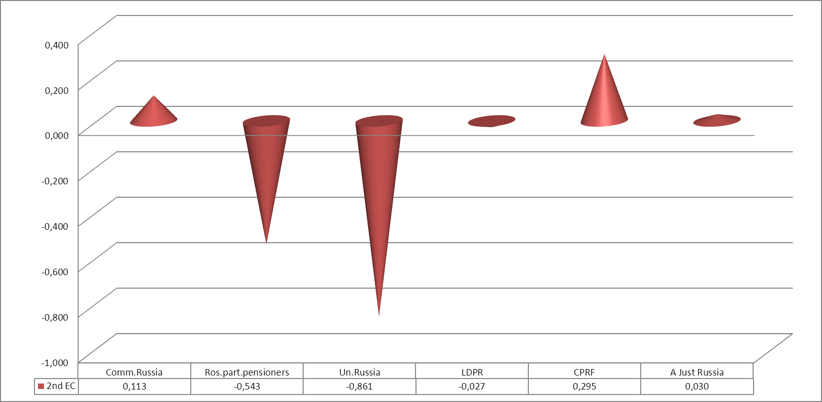
Figure 8. Second political dimension in the regions displaying the "Parliamentary parties + Communists of Russia + RPPSJ" combination during the 2016 legislative election.
Table 14. Issues with highest factor scores during the 2016 legislative election in the regions displaying the "Parliamentary parties + Communists of Russia + RPPSJ" combination upon second dimension
| Issue | CR | RPPSJ | UR | LDRP | CPRF | AJR | Factor scores |
| Support for Putin | 3 | 5 | 5 | 4 | -3 | 5 | -2.31 |
| Russian Academy of Sciences (RAS) reform | -5 | 0 | 5 | 4 | -5 | -5 | -1.62 |
| Increasing military expenditure | 4 | 5 | 4 | 5 | 5 | 4 | -1.613 |
| The government's efficiency in crisis response | -5 | 0 | 5 | -5 | -5 | -4 | -1.554 |
| Attitude to B. Yeltsin | -5 | 0 | 5 | -5 | -5 | -1 | -1.533 |
| Support for Donetsk and Luhansk People's Republics | 5 | 4 | 5 | 5 | 5 | 5 | -1.528 |
| “Eurasian integration strengthens Russia’s position” | 5 | 4 | 5 | 3 | 5 | 5 | -1.515 |
| … | … | … | … | … | … | … | |
| Directing state funds straight into real economy | 5 | 0 | -5 | 5 | 5 | 5 | 1.02 |
| “Russia’s annexation of Crimea was a violation of international law” | -5 | -5 | -5 | -5 | -5 | -5 | 1.206 |
| Preventing further privatization of state-owned assets | 5 | -1 | -5 | 4 | 5 | 4 | 1.239 |
| “Putin’s foreign policy is reckless” | -5 | -5 | -5 | -5 | -4 | -5 | 1.271 |
| Abolishing the fee for renovation works of buildings | 5 | -3 | -5 | 5 | 5 | 5 | 1.678 |
| “Russia is governed by authoritarian methods” | 0 | -5 | -5 | 4 | 5 | 3 | 1.981 |
| Degree of opposition (self-evaluation) | 0 | -5 | -5 | 4 | 5 | 4 | 1.988 |
| Abolishing contribution pension system | 5 | -5 | -4 | -4 | 5 | 4 | 2.001 |
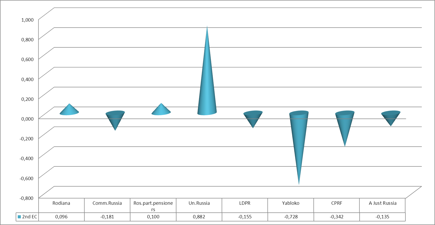
Figure 9. Second political dimension in the regions displaying the "Parliamentary parties + CR + RPPSJ + Yabloko + Rodina" combination during the 2016 legislative election.
Table 15. Issues with highest factor scores during the 2016 legislative election in the regions displaying the "Parliamentary parties + CR + RPPSJ + Yabloko + Rodina" combination upon second dimension
| Issue | Rodina | CR | RPPSJ | UR | LDPR | Yabl | CPRF | AJR | Factor scores |
| Abolishing the fee for renovation works of buildings | 5 | 5 | -3 | -5 | 5 | 5 | 5 | 5 | -1.594 |
| “Russia is governed by authoritarian methods” | -5 | 0 | -5 | -5 | 4 | 5 | 5 | 3 | -1.593 |
| Degree of opposition (self-evaluation) | -3 | 0 | -5 | -5 | 4 | 5 | 5 | 4 | -1.583 |
| Removing municipal filter | 2 | 5 | 0 | -5 | 5 | 5 | 5 | 5 | -1.554 |
| “The Central Bank of Russia and the government are incapable of handling the crisis” | 5 | 5 | 0 | -5 | 5 | 5 | 4 | 4 | -1.422 |
| “The government is using the administrative resource at the elections” | 4 | 4 | 1 | -5 | 5 | 5 | 5 | 2 | -1.386 |
| “The government is destroying small businesses” | 2 | 0 | 0 | -5 | 5 | 5 | 5 | 4 | -1.375 |
| … | … | … | … | … | … | … | |||
| The need to prioritize traditional religious denominations | 4 | -5 | 0 | 5 | 5 | -5 | 5 | 3 | 1.148 |
| Support for Putin | 5 | 3 | 5 | 5 | 4 | -4 | -3 | 5 | 1.396 |
| Attitude to B. Yeltsin | -4 | -5 | 0 | 5 | -5 | -1 | -5 | -1 | 1.54 |
| “Counter-terrorist” Yarovaya law | 3 | 0 | 0 | 5 | -4 | -5 | -4 | 4 | 1.709 |
| Demolishing “unauthorized constructions” | 4 | 0 | 0 | 4 | 1 | -5 | -5 | -4 | 1.709 |
| Russian Academy of Sciences (RAS) reform | -5 | -5 | 0 | 5 | 4 | -5 | -5 | -5 | 1.78 |
| Municipal reform | -1 | 0 | 0 | 5 | -3 | -5 | -5 | -5 | 1.889 |
| The government's efficiency in crisis response | -5 | -5 | 0 | 5 | -5 | -5 | -5 | -4 | 2.007 |
All regions with party combinations ranging from three to five (except Chechnya) generally presented the second political cleavage as socioeconomic with authoritarian-democratic elements as well. Regions with three-dimensional political space repeated the nationwide cleavage hierarchy: 1) systemic ("imperialists"–"anti-imperialists"); 2) authoritarian-democratic; 3) socioeconomic [20: 98–103].
As for the additional political dimensions, the three-party combination produced the "authority–opposition" type variations of authoritarian-democratic and socioeconomic dimensions in all cases as well as the "imperialists"–"anti-imperialists" systemic dimension.
The same list of sub-dimensions persisted in the "four parliamentary parties" combination. The "UR–CPRF–AJR–Communists of Russia" combination (Karachay-Cherkess Republic), "Parliamentary parties + CR" five-party combination and "Parliamentary parties + CR + Patriots of Russia" / "Parliamentary parties + CR + Rodina" / "Parliamentary parties + Patriots of Russia + Rodina" six-party combinations added the "social paternalists vs loyalists" variation of the authoritarian-democratic dimension to this list.
The "Parliamentary parties + CR + RPPSJ" six-party combination added the "communists vs liberals" variation of the socioeconomic dimension to the previous list.
The "Parliamentary parties + CR + RPPSJ + Rodina" seven-party combination brought forward the "government vs opposition" versions of authoritarian-democratic and socioeconomic cleavages, the "conservatives vs liberals" variation of the authoritarian-democratic cleavage and the "communists vs liberals" variation of the socioeconomic cleavage as well as "imperialists vs anti-imperialists" variation of the systemic cleavage.
The "Parliamentary parties + CR + RPPSJ + Party of Growth" seven-party combination (as well as the "Parliamentary parties + Rodina + The Greens + Patriots of Russia" eight-party one) added the "social paternalists vs loyalists" variation of the authoritarian-democratic cleavage while the "Parliamentary parties + CR + RPPSJ + Yabloko" combination (along with "The same + Rodina" eight-party combo and "The same + Rodina + Patriots of Russia" nine-party combo) added the "government vs liberal opposition" variation of the socioeconomic cleavage to the previous list.
The "Parliamentary parties + Rodina + CR + RPPSJ + The Greens + Yabloko" nine-party combination generated all three types of variations for authoritarian-democratic and socioeconomic dimensions as well as the "imperialists vs anti-imperialists" variation of the systemic.
The "Parliamentary parties + Rodina + CR + RPPSJ + Party of Growth + Yabloko" nine-party combination as well as ten- and eleven-party combinations revealed the variations of all three main dimensions.
As for electoral cleavages, most federal subjects displayed either two (31 region, 20 regions less than in 2011) or three (35 regions, three times more than during the previous election). Nine regions (half the 2011 amount) displayed only one cleavage, and eight regions (Saint Petersburg included) displayed four (Table 16).
Table 16. Regions grouped by the number of electoral cleavages during the 2016 elections, a) One cleavage
| Region | Turnout | UR results (%) | No. of parties with >1% votes | No. of PDs | EC-1 | ||||
| Maximum range coef. (Mc) | Effective range coef. (Ec) | Politicization coefficient (Pc) | Socialization coefficient (Sc) | ||||||
| 1 | Kabardino-Balkar Republic | 90.11 | 77.71 | 3 | 1 | 85.31 | 33.04 | 32.97 | 0 |
| 2 | Karachay-Cherkess Republic | 93.32 | 81.67 | 4 | 1 | 91.96 | 23.74 | 23.44 | 0 |
| 3 | Republic of Mordovia | 82.96 | 84.36 | 4 | 1 | 95.75 | 23.88 | 23.44 | 0 |
| 4 | Chechen Republic | 94.92 | 96.29 | 3 | 1 | 93.69 | 3.06 | 3.06 | 0.88 |
| 5 | Belgorod Oblast | 62.38 | 54.655 | 6 | 1 | 88.35 | 68.68 | 67.04 | 23.93 |
| 6 | Kemerovo Oblast | 86.76 | 77.31 | 4 | 1 | 90.31 | 29.48 | 28.84 | 6.41 |
| 7 | Lipetsk Oblast | 52.62 | 56.005 | 7 | 1 | 89.13 | 67.36 | 67.08 | 40.96 |
| 8 | Penza Oblast | 60.57 | 64.3 | 6 | 1 | 91.12 | 54.95 | 54.86 | 29.88 |
| 9 | Tyumen Oblast | 81.1 | 58.36 | 4 | 1 | 92.24 | 68.37 | 67.81 | 55.61 |
b) Two cleavages
| Region | Turnout | UR (%) | No. of parties with >1% votes | No. of PDs | EC-1 | EC-2 | |||||||
| Mc | Ec | Pc | Sc | Mc | Ec | Pc | Sc | ||||||
| 1 | Republic of Adygea | 53.87 | 59.45 | 6 | 2 | 81.65 | 48.61 | 45.83* | 0 | 24.25 | 22.27 | 0 | 10.38 |
| 2 | Republic of Dagestan | 88.1 | 88.86 | 3 | 2 | 91.76 | 10.43 | 0 | 0 | 11.77 | 4.44 | 0 | 0.74 |
| 3 | Republic of Kalmykia | 57.5 | 70.61 | 6 | 2 | 87.88 | 35.7 | 33.08 | 18.48 | 9.28 | 7.71 | 0 | 0 |
| 4 | Crimea+Sevastopol | 48.58 | 67.915 | 7 | 2 | 88.56 | 43.69 | 43.68 | 33.71 | 88.56 | 43.69 | 9.17 | 33.71 |
| 5 | Mari El Republic | 53.34 | 46.7 | 6 | 2 | 63.05 | 35.05 | 0 | 37 | 48.19 | 43.66 | 0 | 0 |
| 6 | Tatarstan | 79.34 | 84.845 | 5 | 2 | 92.1 | 17.75 | 17.32 | 14.41 | 19.55 | 5.56 | 0 | 2.2 |
| 7 | Tyva Republic | 89.73 | 82.61 | 4 | 2 | 90.94 | 18.66 | 17.69 | 8.41 | 6.19 | 5.46 | 0 | 1.39 |
| 8 | Udmurt Republic | 44.49 | 50.49 | 6 | 2 | 62.71 | 36.17 | 0 | 32.32 | 42.27 | 31.5 | 0 | 0 |
| 9 | Chuvash Republic | 59.33 | 50.875 | 6 | 2 | 81.7 | 63.8 | 62.88 | 43.15 | 21.98 | 14.33 | 0 | 3.27 |
| 10 | Stavropol Krai | 42.07 | 54.095 | 7 | 2 | 81.41 | 57.39 | 54.01 | 0 | 20.69 | 12.55 | 0 | 8.58 |
| 11 | Bryansk Oblast | 55.14 | 63.905 | 7 | 2 | 88.5 | 51.67 | 50.63 | 13.5 | 9.6 | 7.23 | 0 | 0.93 |
| 12 | Volgograd Oblast | 42.15 | 50.54 | 8 | 2 | 77.3 | 55.4 | 33.78 | 13.67 | 22.64 | 12.61 | 0 | 8.06 |
| 13 | Voronezh Oblast | 53.99 | 58.44 | 7 | 2 | 83.76 | 55.19 | 32.17 | 25.34 | 22.83 | 14.39 | 0 | 1.86 |
| 14 | Kursk Oblast | 46.98 | 51.68 | 8 | 2 | 17.9 | 10.01 | 0 | 5.14 | 17.9 | 10.01 | 5.14 | 5.14 |
| 15 | Nizhny Novgorod Oblast | 41.69 | 57.66 | 7 | 2 | 81.41 | 49.55 | 46.43 | 15.72 | 17.81 | 8.68 | 0 | 4.43 |
| 16 | Novosibirsk Oblast | 35.07 | 38.285 | 8 | 2 | 76.16 | 51.26 | 0 | 39.91 | 24.16 | 23.04 | 13.48 | 0 |
| 17 | Omsk Oblast | 38.77 | 36.07 | 8 | 2 | 67.39 | 55.78 | 0 | 46.12 | 33.8 | 27.31 | 0 | 0 |
| 18 | Orenburg Oblast | 41.63 | 40.415 | 6 | 2 | 59.1 | 42.28 | 37.27* | 13.05 | 35.84 | 31.06 | 0 | 13.99 |
The table is not fully displayed Show table
с) Three cleavages (beginning)
| Region | Turnout | UR (%) | No. of parties with >1% votes | No. of PDs | EC-1 | EC-2 | EC-3 | ||||||||||
| Mc | Ec | Pc | Sc | Mc | Ec | Pc | Sc | Mc | Ec | Pc | Sc | ||||||
| 1 | Altai Republic | 45.1 | 48.81 | 7 | 2 | 81.63 | 66.23 | 0 | 0 | 15.99 | 15.88 | 0 | 0 | 14.65 | 9.96 | 0 | 0 |
| 2 | Republic of Bashkortostan | 69.69 | 56.45 | 6 | 2 | 49.46 | 31.63 | 20.21* | 3.31 | 60.21 | 26.08 | 0 | 2.66 | 31.79 | 19.71 | 0 | 0 |
| 3 | Republic of Buryatia | 40.5 | 43.34 | 7 | 2 | 69.63 | 53.97 | 49.56 | 25.25 | 30.07 | 22.54 | 0 | 15.54 | 17.79 | 13.88 | 0 | 2.64 |
| 4 | Republic of Ingushetia | 81.42 | 72.41 | 8 | 2 | 34.56 | 34.46 | 16.18* | 0 | 76.07 | 16.85 | 7.57* | 11.12 | 25.72 | 5.17 | 3.38 | 0 |
| 5 | Republic of North Ossetia | 85.59 | 67.09 | 6 | 2 | 48.3 | 12.01 | 0 | 0 | 64.46 | 28.44 | 18.62 | 0 | 44.22 | 10.5 | 6.06 | 20.29 |
| 6 | Yakutia Republic | 48.09 | 46.42 | 7 | 2 | 47.51 | 26.35 | 0 | 0 | 48.1 | 33.26 | 21.8 | 4.39 | 40.11 | 20.5 | 0 | 2.37 |
| 7 | Republic of Khakassia | 39.36 | 38.06 | 7 | 2 | 58.75 | 45.14 | 42.6* | 26.07 | 33.14 | 21.79 | 0 | 0 | 12.28 | 11.47 | 0 | 0 |
| 8 | Zabaykalsky Krai | 38.85 | 39.865 | 7 | 2 | 72.73 | 69.77 | 0 | 43.76 | 20.33 | 15 | 0 | 10.01 | 29.22 | 21.9 | 0 | 6.34 |
| 9 | Kamchatka Krai | 39.5 | 46.7 | 7 | 2 | 74.5 | 57.58 | 72.64 | 41.95 | 26.64 | 24.37 | 0 | 0 | 14.73 | 5.8 | 0 | 1.87 |
| 10 | Krasnodar Krai | 51.16 | 46.7 | 9 | 3 | 79.62 | 68.48 | 46.67 | 0 | 13.68 | 6.42 | 4.75 | 4.95 | 18.26 | 15.81 | 0 | 3.41 |
| 11 | Primorsky Krai | 36.14 | 39.01 | 9 | 3 | 50 | 37.13 | 14.28 | 28.65 | 59.46 | 58.86 | 32.71 | 13.94 | 25.08 | 22.17 | 8.19 | 5.28 |
| 12 | Khabarovsk Krai | 36.89 | 37.19 | 9 | 3 | 52.46 | 45 | 24.24 | 40.43 | 51.98 | 49.68 | 23.38 | 26.49 | 17.76 | 13.93 | 0 | |
| 13 | Amur Oblast | 42.4 | 37.91 | 7 | 2 | 68.79 | 66.36 | 62.39 | 49.37 | 32.38 | 28.06 | 15.47 | 0 | 29.19 | 24.02 | 0 | 6.22 |
| 14 | Astrakhan Oblast | 36.85 | 42.22 | 7 | 2 | 58.05 | 49.79 | 0 | 24.7 | 48.25 | 31.29 | 0 | 25.2 | 24.64 | 18.48 | 0 | 16.47 |
| 15 | Vladimir Oblast | 38.35 | 45.165 | 9 | 3 | 67.75 | 40.83 | 17.27* | 35.07 | 31.3 | 21.54 | 7.82 | 7.82 | 31.38 | 31.28 | 15.2 | 10.63 |
| 16 | Ivanovo Oblast | 38.51 | 42.26 | 8 | 2 | 79.47 | 75.24 | 51.33 | 51.88 | 23.31 | 13.24 | 0 | 10.37 | 10.38 | 10.36 | 4.48 | 0 |
| 17 | Irkutsk Oblast | 34.59 | 39.715 | 7 | 2 | 54.26 | 38.27 | 31.88* | 30.61 | 36.21 | 32.97 | 15.59* | 21.87 | 43.37 | 42.53 | 22.34 | 4.46 |
| 18 | Kaliningrad Oblast | 44.01 | 43.39 | 10 | 3 | 60.98 | 46.05 | 33.15 | 33.28 | 47.29 | 47.13 | 17.7* | 16.86 | 15.34 | 8.99 | 0 | 0 |
(end)
| Region | Turnout | UR (%) | No. of parties with >1% votes | No. of PDs | EC-1 | EC-2 | EC-3 | ||||||||||
| Mc | Ec | Pc | Sc | Mc | Ec | Pc | Sc | Mc | Ec | Pc | Sc | ||||||
| 19 | Kaluga Oblast | 43.07 | 45.715 | 8 | 2 | 56.89 | 34.05 | 0 | 30.1 | 31.58 | 20.89 | 0 | 8.94 | 46.57 | 39.35 | 27.54 | 0 |
| 20 | Kirov Oblast | 40.69 | 37.91 | 7 | 2 | 59.11 | 42.43 | 0 | 28.58 | 44.4 | 27.22 | 14.65* | 14.51 | 35.08 | 30.58 | 23.13 | 3.32 |
| 21 | Kostroma Oblast | 39.36 | 36.56 | 8 | 2 | 41.98 | 19.99 | 0 | 13.02 | 51.17 | 39.34 | 19.24 | 0 | 39.92 | 34.61 | 0 | 5.39 |
| 22 | Kurgan Oblast | 41.82 | 41.51 | 7 | 2 | 56.74 | 39.41 | 0 | 33.64 | 45.26 | 35.2 | 0 | 12.38 | 29.15 | 24.91 | 0 | 5.83 |
| 23 | Leningrad Oblast | 44.12 | 50 | 8 | 2 | 70.5 | 50.42 | 34.16 | 0 | 18.45 | 13.01 | 0 | 10.63 | 35.11 | 18.41 | 0 | 7.06 |
| 24 | Magadan Oblast | 40.55 | 44.69 | 7 | 2 | 64.73 | 59.84 | 53.12 | 0 | 33.44 | 31.91 | 0 | 18.61 | 36.78 | 17.61 | 15.55 | 0 |
| 25 | Moscow Oblast | 38.06 | 45.82 | 11 | 3 | 54.39 | 36.16 | 25.76 | 13.23 | 53.58 | 45.19 | 32.87 | 14.52 | 26.78 | 25 | 4.9 | |
| 26 | Murmansk Oblast | 39.67 | 41.98 | 8 | 2 | 71.33 | 45.66 | 21.97* | 32.07 | 14.5 | 8.93 | 0 | 0 | 29.08 | 25.99 | 13.8 | 0 |
| 27 | Novgorod Oblast | 39.85 | 40.05 | 8 | 3 | 67.82 | 47.8 | 29.45 | 38.84 | 37.19 | 35.82 | 0 | 0 | 24.65 | 23.14 | 14.74 | 6.11 |
| 28 | Pskov Oblast | 42.09 | 45.15 | 8 | 2 | 64.91 | 44.46 | 30.27 | 17.63 | 26.88 | 15.77 | 0 | 7.44 | 16.32 | 13.56 | 0 | 2.92 |
| 29 | Sakhalin Oblast | 37.06 | 45.44 | 8 | 2 | 64.85 | 44.43 | 29.74 | 30.87 | 30.98 | 28.29 | 0 | 19.12 | 20.73 | 20.64 | 0 | 11.03 |
| 30 | Sverdlovsk Oblast | 41.46 | 40.56 | 9 | 3 | 55.42 | 34.3 | 12.09* | 25.92 | 40.24 | 32.9 | 17.61 | 8.25 | 20.85 | 14.34 | 0 | 1.93 |
| 31 | Smolensk Oblast | 40.23 | 47.815 | 8 | 2 | 64.19 | 39.45 | 34.31 | 25.67 | 35.34 | 30.38 | 19.39 | 8.73 | 28.33 | 23.93 | 0 | 3.29 |
| 32 | Chelyabinsk Oblast | 44.42 | 38.148 | 8 | 2 | 56.83 | 36.18 | 0 | 29.02 | 37.72 | 32.27 | 0 | 9.69 | 24.56 | 22.35 | 0 | 10.02 |
| 33 | Yaroslavl Oblast | 37.76 | 38.46 | 10 | 3 | 73.14 | 47.12 | 0 | 43.89 | 32.72 | 29.1 | 0 | 0 | 23.24 | 22.42 | 0 | 0 |
| 34 | Moscow | 35.25 | 37.72 | 11 | 3 | 68.26 | 50.17 | 26.56 | 29.14 | 37.65 | 33.87 | 13.5 | 4.46 | 15.43 | 10.77 | 0 | 0.95 |
| 35 | Khanty-Mansi AO | 39.35 | 47.08 | 9 | 3 | 80.82 | 68.97 | 43.12 | 36.17 | 14.68 | 14.34 | 11.29 | 11.79 | 16.51 | 14.37 | 8 | 5.54 |
d) Four cleavages
| EC-1 | EC-2 | EC-3 | EC-4 | |||||||||||||||||
| Region | Turnout | UR (%) | No. of pts (> 1%) | No. of PDs | Mc | Ec | Pc | Sc | Mc | Ec | Pc | Sc | Mc | Ec | Pc | Sc | Mc | Ec | Pc | Sc |
| Republic of Karelia | 39.59 | 37.3 | 9 | 3 | 45.8 | 21.77 | 19.62 | 20.48 | 45.17 | 30.43 | 30.13 | 13.74 | 24.78 | 20.49 | 0 | 6.22 | 29.78 | 22.52 | 0 | 0 |
| Komi Republic | 40.75 | 37.85 | 8 | 2 | 50.36 | 29.57 | 16.5 | 16.66 | 44.13 | 39.05 | 0 | 24.57 | 11.12 | 9.87 | 0 | 2.7 | 24.15 | 19.05 | 0 | 6.18 |
| Altai Krai | 40.82 | 35.195 | 7 | 2 | 34.87 | 23.05 | 0 | 5.28 | 50.1 | 38.32 | 21.41* | 10.74 | 29.27 | 22.72 | 0 | 6.48 | 18.72 | 14.16 | 10.96 | 1.01 |
| Krasnoyarsk Krai | 36.61 | 40.816 | 9 | 2 | 51.06 | 29.57 | 25.61 | 22.92 | 54.58 | 54.47 | 0 | 20.52 | 9.04 | 8.32 | 0 | 0.88 | 15.45 | 14.07 | 3.45 | 3.45 |
| Perm Krai | 35.09 | 42.66 | 9 | 3 | 48.15 | 25.86 | 16.49* | 20.73 | 33.05 | 29.26 | 19.45 | 0 | 43.99 | 34.3 | 15.31 | 5.35 | 20.23 | 20.15 | 0 | 0 |
| Arkhangelsk Oblast + Nenets AO | 39.27 | 44.44 | 9 | 3 | 62.65 | 42.4 | 32.81* | 29.79 | 21.29 | 16.9 | 14.28 | 11.45 | 32.97 | 29.57 | 0 | 9.99 | 30.74 | 30.65 | 0 | 7.33 |
| Vologda Oblast | 40.82 | 37.4 | 8 | 2 | 58.89 | 41.83 | 0 | 17.42 | 49.42 | 31.77 | 0 | 0 | 22.37 | 22.32 | 0 | 7.1 | 21.08 | 16.63 | 0 | 4.44 |
| Saint-Petersburg | 32.49 | 39.72 | 11 | 3 | 54.77 | 33.36 | 13.09 | 18.96 | 52.77 | 47.33 | 33.08 | 13.07 | 13.26 | 11.67 | 0 | 1.87 | 20.78 | 19.62 | 10 | 2.52 |
* Correlation coefficient with a ≤10% margin of error. In the remaining cases the margin of error is <5%.
The number of parties with >1% vote count fluctuated from three (Kabardino-Balkaria) to seven (Lipetsk Oblast) in the one-EC group. This group also registered the highest voter turnout and the highest electoral cleavage maximum range coefficients. The effective range, politicization and socialization coefficients for this EC ranged very broadly.
The group with four electoral cleavages displayed a reverse fluctuation in the number of parties with >1% vote count: from seven in Altai Krai to eleven in Saint Petersburg. The turnout never went over 41% in any region, the maximum range coefficient for the first EC was moderate, the effective range coefficient fluctuated from 21.8 (Karelia) to 42.4 (Arkhangelsk Oblast with Nenets AO); politicization and socialization coefficients were quite low but present almost everywhere. The second EC had a political interpretation in most cases; the third EC was politically coloured only in Perm Krai while the fourth one was political in three cases out of eight. Only Saint-Petersburg stands out, where three out of four ECs had a political content.
The group with two electoral cleavages was characterized by a high maximum range coefficient (except for Kursk Oblast), and high variation in effective range, politicization and socialization coefficients for the first EC. The second EC as a rule displayed much lower maximum and effective range coefficients as well as socialization coefficient, while also rarely indicating any political interpretation.
In the group with three electoral cleavages, each of them generally lacked any political interpretation while the margin of error for the correlation with political dimensions fluctuated between 5 and 10% in most cases. At the same time, all three electoral cleavages mostly had a social background while the first EC in fact displayed quite high socialization and effective range coefficients.
Sorting the first cleavage by the maximum range coefficient expectedly put forward several republics (Mordovia, Chechnya, Tatarstan, Karachay-Cherkessia, Dagestan and Tyva) and oblasts (Tomsk, Penza and Chelyabinsk). The republics of North Caucasus as well as Tyva, Tatarstan and Mordovia registered the lowest balance ratio coefficient values for the sides of the authoritarian-democratic cleavage; on the other hand, the same coefficient was highest (>0.9) in Amur, Irkutsk and Ivanovo Oblasts as well as Zabaykalsky Krai.
Zero markers for socialization coefficient were registered not only in North Caucasus, but also in the Far Eastern (Jewish Autonomous Oblast, Chukotka Autonomous Okrug, Magadan Oblast) and Southern (Rostov Oblast, Krasnodar and Stavropol Krais) Federal Districts and even in Leningrad Oblast. On the other hand, such vastly different Oblasts as Ivanovo, Tomsk, Tyumen and Ulyanovsk came to the fore with a coefficient of >50.
The hierarchical tree built via cluster analysis (Figure 10) allowed us to identify two and six primary clusters on various cut-off levels.
Figure 10. Hierarchical tree built via cluster analysis based on structure characteristics of electoral cleavages in the regions during the 2016 legislative election.
The combination of cluster features resulted in identification of six primary groups of regions (Table 17).
Table 17. Regions clustered by political content of electoral cleavages following the 2016 elections (list of political cleavages is incomplete), a) Cluster 1
| EC-1 | EC-2 | EC-3 | |||||||||||||||
| Cl No. (2) | Cl No. (6) | Dist (6) | Region | UR (%) | No. of ECs | Pc | Syst | SE-ASO | SE-CL | Syst-IA | Sc | Pc | SE-CL | Sc | Pc | AD-LL | Sc |
| 2 | 1 | 0.63 | Rostov Oblast | 58.21 | 2 | 44.52 | 0.771 | 0.882 | 0 | 0 | 5.27 | - | - | ||||
| 2 | 1 | 0.64 | Tambov Oblast | 63.41 | 2 | 45.45 | 0.978 | 0 | 0 | 6.51 | - | - | |||||
| 2 | 1 | 0.84 | Republic or Adygea | 59.45 | 2 | 45.83* | 1.156* | 0.642* | 0 | 0 | 10.38 | - | - | ||||
| 2 | 1 | 1.26 | Saratov Oblast | 68.08 | 2 | 35.08* | 1.121* | 0.594* | 3.24 | 0 | 6.83 | - | - | ||||
| 2 | 1 | 1.37 | Krasnodar Krai | 46.7 | 3 | 46.67 | 0.825 | 0 | 4.75 | 0.86 | 0 | 0 | 3.41 | ||||
| 2 | 1 | 1.54 | Stavropol Krai | 54.1 | 2 | 54.01 | 0.761 | 1.343 | 0.63 | 0 | 0 | 8.58 | - | - | |||
| 2 | 1 | 1.69 | Nizhny Novgorod Oblast | 57.66 | 2 | 46.43 | 0.799 | 1.296 | 0.532 | 15.72 | 0 | 4.43 | - | - | |||
| 2 | 1 | 1.79 | Bryansk Oblast | 63.91 | 2 | 50.63 | 1.162 | 0.556 | 13.5 | 0 | 0.93 | - | - | ||||
| 2 | 1 | 1.82 | Leningrad Oblast | 50 | 3 | 34.16 | 0.823 | 0 | 0 | 10.63 | 0 | 7.06 | |||||
| 2 | 1 | 1.87 | Orenburg Oblast | 40.42 | 2 | 37.27* | 1.118* | 0.600* | 13.05 | 0 | 13.99 | - | - | ||||
| 2 | 1 | 1.88 | Kabardino-Balkar Republic | 77.71 | 1 | 32.97 | 0 | - | - | - | - | ||||||
| 2 | 1 | 1.97 | Volgograd Oblast | 50.54 | 2 | 33.78 | 13.67 | 0 | 8.06 | - | - | ||||||
| 2 | 1 | 2.02 | Chukotka AO | 58.8 | 2 | 56.21 | 0.807 | 0.987 | 0.499 | 0 | 0 | 0 | - | - | |||
| 2 | 1 | 2.22 | Jewish AO | 45.03 | 2 | 58.72 | 1.153 | 0.53 | 0 | 0 | 11.16 | - | - | ||||
| 2 | 1 | 2.32 | Kemerovo Oblast | 77.31 | 1 | 28.84 | 0.989 | 6.41 | - | - | - | - | |||||
| 2 | 1 | 2.98 | Magadan Oblast | 44.69 | 3 | 53.12 | 0.93 | 0 | 0 | 18.61 | 15.55 | 0.939 | 0 | ||||
b) Cluster 2
| EC-1 | EC-2 | EC-3 | ||||||||||||||
| Cl No. (2) | Cl No. (6) | Dist (6) | Region | UR (%) | No. of ECs | Pc | AD | Sc | Pc | Syst | SE | SE-CL | Sc | Pc | SE-ASO | Sc |
| 1 | 2 | 0.95 | Kursk Oblast | 51.68 | 2 | 0 | 36.31 | 5.14 | 0.749 | 5.14 | - | - | ||||
| 1 | 2 | 1.18 | Kurgan Oblast | 41.51 | 3 | 0 | 33.64 | 0 | 12.38 | 0 | 5.83 | |||||
| 1 | 2 | 1.45 | Mari El Republic | 46.7 | 2 | 0 | 37 | 0 | 0 | - | - | |||||
| 1 | 2 | 1.46 | Udmurt Republic | 50.49 | 2 | 0 | 32.32 | 0 | 0 | - | - | |||||
| 1 | 2 | 1.51 | Chelyabinsk Oblast | 38.15 | 3 | 0 | 29.02 | 0 | 9.69 | 0 | 10.02 | |||||
| 1 | 2 | 1.61 | Zabaykalsky Krai | 39.87 | 3 | 0 | 43.76 | 0 | 10.01 | 0 | 6.34 | |||||
| 1 | 2 | 1.89 | Yaroslavl Oblast | 38.46 | 3 | 0 | 43.89 | 0 | 0 | 0 | 0 | |||||
| 1 | 2 | 1.91 | Tomsk Oblast | 40.71 | 2 | 0 | 27.32 | 13.66 | 0.686 | 6.72 | - | - | ||||
| 1 | 2 | 2 | Novosibirsk Oblast | 38.29 | 2 | 0 | 39.91 | 13.48 | 0.765 | 0 | - | - | ||||
| 1 | 2 | 2.11 | Omsk Oblast | 36.07 | 2 | 0 | 46.12 | 0 | 0 | - | - | |||||
| 1 | 2 | 2.88 | Vladimir Oblast | 45.17 | 3 | 17.27* | 0.65* | 35.07 | 7.82 | 7.82 | 15.2 | 0.697 | 10.63 | |||
| 1 | 2 | 3.26 | Kirov Oblast | 37.91 | 3 | 0 | 28.58 | 14.65* | 0.734* | 14.51 | 23.13 | 0.87 | 3.32 | |||
| 1 | 2 | 3.34 | Kaluga Oblast | 45.72 | 3 | 0 | 30.1 | 0 | 8.94 | 27.54 | 0.837 | 0 | ||||
| 1 | 2 | 3.48 | Astrakhan Oblast | 42.22 | 3 | 0 | 24.7 | 0 | 25.2 | 0 | 16.47 | |||||
c) Cluster 3
| EC-1 | EC-2 | EC-3 | ||||||||||||||
| Cl No. (2) | Cl No. (6) | Dist (6) | Region | UR (%) | No. of ECs | Pc | Syst | SE-ASO | SE-CL | Sc | Pc | SE-CL | Sc | Pc | SE-CL | Sc |
| 2 | 3 | 0.38 | Chuvash Republic | 50.88 | 2 | 62.88 | 1.438 | 0.771 | 43.15 | 0 | 3.27 | 0 | 0 | |||
| 2 | 3 | 0.82 | Lipetsk Oblast | 56.01 | 1 | 67.08 | 0.796 | 1.373 | 0.496 | 40.96 | - | - | - | - | ||
| 2 | 3 | 1.25 | Samara Oblast | 50.25 | 2 | 66.45 | 42.78 | 10* | 1.249 | 5.61 | - | - | ||||
| 2 | 3 | 1.45 | Kamchatka Krai | 46.7 | 3 | 72.64 | 0.93 | 0.106 | 41.95 | 0 | 0 | 0 | 1.87 | |||
| 2 | 3 | 1.98 | Tyumen Oblast | 58.36 | 1 | 67.81 | 0.996 | 0.996 | 55.61 | - | - | - | - | |||
| 2 | 3 | 2.19 | Penza Oblast | 64.3 | 1 | 54.86 | 0.817 | 1.313 | 0.339 | 29.88 | - | - | - | 0 | ||
| 2 | 3 | 2.22 | Amur Oblast | 37.91 | 3 | 62.39 | 0.851 | 1.3 | 0.535 | 49.37 | 15.47 | 0.743* | 0 | 0 | 6.22 | |
| 2 | 3 | 2.41 | Ivanovo Oblast | 42.26 | 3 | 51.33 | 51.88 | 0 | 10.37 | 4.48 | 0.658* | 0 | ||||
| 2 | 3 | 2.69 | Ryazan Oblast | 54.51 | 2 | 63.14 | 0.791 | 1.356 | 0.63 | 23.67 | 0 | 5.46 | - | - | ||
| 2 | 3 | 2.72 | Belgorod Oblast | 54.66 | 1 | 67.04 | 1.169 | 23.93 | - | - | - | - | ||||
| 2 | 3 | 3.52 | Ulyanovsk Oblast | 47.64 | 2 | 58.13 | 66.96 | 0.16 | 8.09 | - | - | |||||
d) Cluster 4
| EC-1 | EC-2 | EC-3 | EC-4 | |||||||||||||
| Cl No. (2) | Cl No. (6) | Dist (6) | Region | UR (%) | No. of ECs | Pc | AD-GO | SE-ASO | Sc | Pc | SE-CL | Sc | Pc | Sc | Pc | Sc |
| 2 | 4 | 1.13 | Voronezh Oblast | 58.44 | 2 | 32.17 | 0.763 | 25.34 | 0 | 1.86 | - | - | - | - | ||
| 2 | 4 | 1.29 | Yamalo-Nenets AO | 67.14 | 2 | 30.07* | 0.853* | 27.34 | 0 | 0 | - | - | - | - | ||
| 2 | 4 | 1.59 | Republic of Khakassia | 38.06 | 3 | 42.60* | 1.453* | 26.07 | 0 | 0 | 0 | 0 | 0 | 0 | ||
| 2 | 4 | 1.7 | Crimea+Sevastopol | 67.92 | 2 | 43.68 | 0.12 | 1.197 | 33.71 | 9.17 | 2.56 | - | - | - | - | |
| 2 | 4 | 1.85 | Tula Oblast | 53 | 2 | 30.75 | 0.741 | 41.09 | 0 | 2.24 | - | - | - | - | ||
| 1 | 4 | 1.88 | Moscow | 37.72 | 3 | 26.56 | 0.662 | 29.14 | 13.5 | 4.46 | 0 | 0.95 | 0 | 0 | ||
| 2 | 4 | 1.92 | Republic of Kalmykia | 70.61 | 2 | 33.08 | 0.946 | 18.48 | 0 | 0 | - | - | - | - | ||
| 2 | 4 | 1.92 | Pskov Oblast | 45.15 | 3 | 30.27 | 0.825 | 17.63 | 0 | 7.44 | 0 | 2.92 | - | - | ||
| 2 | 4 | 2.03 | Tver Oblast | 44.83 | 2 | 44.4 | 0.805 | 38.8 | 8.13 | 0.731 | 2.6 | - | - | - | - | |
| 2 | 4 | 2.07 | Arkhangelsk Oblast + Nenets AO | 44.44 | 4 | 32.81* | 0.880* | 29.79 | 14.28 | 1.384 | 11.45 | 0 | 9.99 | 0 | 7.33 | |
| 2 | 4 | 2.21 | Khanty-Mansi AO | 47.08 | 3 | 43.12 | 0.791 | 36.17 | 11.29 | 1.327 | 11.79 | 8 | 5.54 | - | - | |
| 2 | 4 | 2.25 | Oryol Oblast | 47.93 | 2 | 47.52* | 3.544* | 4.244* | 35.01 | 0 | 0 | - | - | - | - | |
| 2 | 4 | 2.39 | Sakhalin Oblast | 45.44 | 3 | 29.74 | 0.818 | 30.87 | 0 | 19.12 | 0 | 11.03 | - | - | ||
| 2 | 4 | 2.52 | Novgorod Oblast | 40.05 | 3 | 29.45 | 0.785 | 38.84 | 0 | 0 | 14.74 | 6.11 | - | - | ||
| 1 | 4 | 2.59 | Murmansk Oblast | 41.98 | 3 | 21.97* | 0.645* | 32.07 | 0 | 13.8 | 0 | - | - | |||
| 2 | 4 | 2.63 | Republic of Buryatia | 43.34 | 3 | 49.56 | 0.91 | 25.25 | 0 | 15.54 | 0 | 2.64 | - | - | ||
| 1 | 4 | 2.66 | Krasnoyarsk Krai | 40.82 | 4 | 25.61 | 0.343 | 0.343 | 22.92 | 0 | 20.52 | 0 | 0.88 | 3.45 | 3.45 | |
e) Cluster 5
| EC-1 | EC-2 | EC-3 | EC-4 | ||||||||||||||
| Cl No. (2) | Cl No. (6) | Dist (6) | Region | UR (%) | No. of ECs | Pc | AD | AD-GO | SE-CL | Sc | Pc | SE-ASO | Sc | Pc | Sc | Pc | Sc |
| 1 | 5 | 1.42 | Republic of Karelia | 37.3 | 4 | 19.62 | 0.624 | 0.196 | 0.287 | 20.48 | 30.13 | 0.784 | 13.74 | 0 | 6.22 | 0 | 0 |
| 1 | 5 | 1.79 | Primorsky Krai | 39.01 | 3 | 14.28 | 0.62 | 0.586 | 28.65 | 32.71 | 0.746 | 13.94 | 8.19 | 5.28 | - | - | |
| 1 | 5 | 1.99 | Sverdlovsk Oblast | 40.56 | 3 | 12.09* | 0.594* | 25.92 | 17.61 | 0.732 | 8.25 | 0 | 1.93 | - | - | ||
| 2 | 5 | 2.01 | Smolensk Oblast | 47.82 | 3 | 34.31 | 0.692 | 25.67 | 19.39 | 8.73 | 0 | 3.29 | - | - | |||
| 1 | 5 | 2.15 | Saint-Petersburg | 39.72 | 4 | 13.09 | 0.626 | 18.96 | 33.08 | 0.836 | 13.07 | 0 | 1.87 | 10 | 2.52 | ||
| 2 | 5 | 2.21 | Kaliningrad Oblast | 43.39 | 3 | 33.15 | 0.727 | 0.848 | 33.28 | 17.7* | 0.613 | 16.86 | 0 | 0 | - | - | |
| 1 | 5 | 2.28 | Moscow Oblast | 45.82 | 3 | 25.76 | 0.703 | 1.039 | 13.23 | 32.87 | 0.853 | 14.52 | 0 | 4.9 | - | - | |
| 1 | 5 | 2.75 | Perm Krai | 42.66 | 4 | 16.49* | 0.663* | 0.637* | 0.494* | 20.73 | 19.45 | 0 | 15.31 | 5.35 | 0 | 0 | |
| 1 | 5 | 2.82 | Khabarovsk Krai | 37.19 | 3 | 24.24 | 0.734 | 40.43 | 23.38 | 0.686 | 26.49 | 0 | 0 | - | - | ||
| 2 | 5 | 3.31 | Irkutsk Oblast | 39.72 | 3 | 31.88* | 0.886* | 30.61 | 15.59* | 21.87 | 22.34 | 4.46 | - | - | |||
f) Cluster 6
| EC-1 | EC-2 | EC-3 | EC-4 | |||||||||||||||
| Cl No. (2) | Cl No. (6) | Dist (6) | Region | UR (%) | No. of ECs | Pc | Syst | SE-ASO | Sc | Pc | AD-GO | Sc | Pc | Syst-IA | Sc | Pc | AD-GO | Sc |
| 1 | 6 | 1.5 | Chechen Republic | 96.29 | 1 | 3.06 | 0.997 | 1 | 0.88 | - | - | - | - | - | - | |||
| 1 | 6 | 1.6 | Tyva Republic | 82.61 | 2 | 17.69 | 0.974 | 0.973 | 8.41 | 0 | 1.39 | - | - | - | - | |||
| 1 | 6 | 1.7 | Republic of Ingushetia | 72.41 | 3 | 16.18* | 0 | 7.57* | 0.671* | 11.12 | 3.38 | 0.809 | 0 | - | - | |||
| 1 | 6 | 1.79 | Republic of Dagestan | 88.86 | 2 | 0 | 0 | 0 | 0.74 | - | - | - | - | |||||
| 1 | 6 | 1.82 | Altai Republic | 48.81 | 3 | 0 | 0 | 0 | 0 | 0 | 0 | - | - | |||||
| 1 | 6 | 1.82 | Republic of Bashkortostan | 56.45 | 3 | 20.21* | 3.31 | 0 | 2.66 | 0 | 0 | - | - | |||||
| 1 | 6 | 1.95 | Republic of Tatarstan | 84.85 | 2 | 17.32 | 0.988 | 14.41 | 0 | 2.2 | - | - | - | - | ||||
| 1 | 6 | 2.36 | Republic of Mordovia | 84.36 | 1 | 23.44 | 0.991 | 0 | - | - | - | - | - | - | ||||
| 1 | 6 | 2.36 | Karachay-Cherkess Republic | 81.67 | 1 | 23.44 | 0.994 | 0 | - | - | - | - | - | - | ||||
| 1 | 6 | 2.4 | Vologda Oblast | 37.4 | 4 | 0 | 17.42 | 0 | 0 | 0 | 7.1 | 0 | 4.44 | |||||
| 1 | 6 | 2.57 | Kostroma Oblast | 36.56 | 3 | 0 | 13.02 | 19.24 | 0.699* | 0 | 0 | 5.39 | - | - | ||||
| 1 | 6 | 2.66 | Yakutia Republic | 46.42 | 3 | 0 | 0 | 21.8 | 4.39 | 0 | 2.37 | - | - | |||||
| 1 | 6 | 2.72 | Altai Krai | 35.2 | 4 | 0 | 5.28 | 21.41* | 10.74 | 0 | 6.48 | 10.96 | 0.774 | 1.01 | ||||
| 1 | 6 | 3.45 | Republic of North Ossetia | 67.09 | 3 | 0 | 0 | 18.62 | 0 | 6.06 | 20.29 | - | - | |||||
| 1 | 6 | 3.53 | Komi Republic | 37.85 | 4 | 16.5 | 16.66 | 0 | 24.57 | 0 | 2.7 | 0 | 6.18 | |||||
Types of political cleavages related to the corresponding electoral cleavage (disambiguation):
AD – Authoritarian-democratic
SE – Socioeconomic
Syst – Systemic
AD-GO – Authoritarian-democratic (government vs opposition)
AD-LL – Authoritarian-democratic (liberals vs loyalists)
AD-SPL – Authoritarian-democratic (social patriots vs loyalists)
SE-ASO – Socioeconomic (government vs systemic opposition)
SE-CL – Socioeconomic (communists vs liberals)
SE-ALO – Socioeconomic (government vs liberal opposition)
Syst-IA – Systemic ("imperialists" vs "anti-imperialists")
Syst-SL – Systemic (statists vs liberals)
* Correlation coefficient with a ≤10% margin of error. In the remaining cases the margin of error is <5%.
The first cluster was comprised of 16 regions (with Rostov Oblast, Tambov Oblast and the Republic of Adygea in the center) with average politicization coefficient values (mainly connected with the "government vs systemic opposition" variation of socioeconomic dimension) and low or zero socialization coefficient values. The number of votes for United Russia fluctuates from average to high; the number of electoral cleavages fluctuates from one to three.
The main feature of the second cluster (14 regions with Kursk and Kurgan Oblasts in the center) is the lack of political interpretation (or the weak connection to political dimensions with a >10% margin of error, to be more exact) in the first electoral cleavage which in its turn has quite high socialization coefficients. The number of votes for United Russia is moderate; the number of electoral cleavages is two or three.
The third cluster is comprised of 11 regions (with Chuvash Republic and Lipetsk Oblast in the center) where the first electoral cleavage has connection to a variation of socioeconomic and systemic dimensions. Politicization and socialization coefficients of the first EC are quite high. The number of votes for United Russia is closer to average; the number of electoral cleavages ranges from one to three.
The fourth cluster is comprised of 17 regions (with Voronezh Oblast, Yamalo-Nenets AO and Khakassia in the center). In this case, the first electoral cleavage is connected to the "government vs opposition" variation of authoritarian-democratic and socioeconomic dimensions. Politicization and socialization coefficients are lower than in the previous cluster while the number of votes for United Russia is higher; the number of electoral cleavage ranges from two to four.
The fifth cluster (10 regions with Karelia, Primorsky Krai and Sverdlovsk Oblast in the center) is characterized by a low number of votes for United Russia, a high number of electoral cleavages (three to four), low politicization and socialization coefficients for the first electoral cleavage which is connected to authoritarian-democratic dimension variations and the "communists vs liberals" variation of the socioeconomic dimension. The second EC revealed political content (mostly the "government vs systemic opposition" variation of the socioeconomic dimension) and social background in this cluster.
The sixth, and final, cluster (15 regions with Chechnya and Tyva in the center) indicated low (or zero) politicization and socialization coefficient values and a high number of votes for United Russia (with the exception of Vologda and Kostroma Oblasts, Komi Republic and Altai Krai). The first EC presented little political content which was mostly systemic. This cluster is possibly the least competitive, although the regions with high competitiveness levels (which are part of this cluster) should not be overlooked.
Cluster analysis results for this election generally display a weaker connection to a competitiveness level than for the 2011 election. In this case, it is also much more difficult to identify explicitly competitive and non-competitive clusters. We can identify prevailing trends only. As a result, the sixth cluster has the lowest number of competitive regions while for the fifth it is quite the opposite with the highest level of competition. The second and third clusters are more disposed towards the fifth while the first has a disposition for the sixth.
At the same time, the "the higher the competition, the more blurred the political landscape in voter consciousness" trend that manifested five years ago persisted. In fact, it became more pronounced. Compared to 2011, even the least competitive regions (ethnic republics, especially those in North Caucasus) presented a more complicated political landscape while the number of regions where the electoral cleavages with social background had little connection to the political dimensions (cluster No. 2) increased manifold.
This could have been explained by the increased number of campaigners, although it is important to remember that the number of parties with >1% vote count had increased almost everywhere as well. This can indicate a certain amount of weakening in administrative pressure applied to voters.
Compared to 2011, Kremlin clearly intended to carry out the 2016 election at a low profile without trying to desperately boost the turnout, which is why it relegated control over this matter to regional governments: the administrative resource continued to prosper in the federal subjects where such circumstances were par for the course while the regions where doing so was fraught with scandals decided not to push it too far. To check this hypothesis, we shall compare the election results in 2011 and 2016 while first focusing on the electoral cleavage measurement tools introduced before (maximum range coefficient, effective range coefficient, politicization coefficient and socialization coefficient).
Table 18 displays the results of comparing regional cleavage structures concerning the decrease or increase in administrative pressure in 2011 and 2016. As we can see, most federal subjects display either a slight decrease in administrative pressure (41) or no changes/contradictory trends (38). Contradictory trends are, on the one hand, a drop in voter turnout and decreased maximum range coefficient for the main cleavage, and decreased effective range, politicization and socialization coefficients on the other. In other words, not only administrative pressure was decreased, but also the level of competition.
Table 18. Decrease/increase trends in administrative pressure in regions of Russia during the 2016 legislative election (as compared to 2011)
| Trend | No. of regions | Regions |
| Significant decrease | 3 | Ingushetia, Komi Republic, Moscow |
| Slight decrease | 41 | Republics: Adygea, Altai, Bashkortostan, Buryatia, Dagestan, Kalmykia, Karelia, Mari El, Tatarstan, Khakassia, Chechnya, Yakutia; Krais: Altai, Zabaykalsky, Kamchatka, Krasnodar, Krasnoyarsk, Perm, Primorky, Khabarovsk; Oblasts: Amur, Arkhangelsk with Nenets Autonomous Okrug, Astrakhan, Vladimir, Voronezh, Irkutsk, Kaliningrad, Kaluga, Kurgan, Novgorod, Omsk, Pskov, Saratov, Sakhalin, Sverdlovsk, Smolensk, Tula, Ulyanovsk, Chelyabinsk; Saint-Petersburg, Khanty-Mansi Autonomous Okrug |
| No changes or contradictory trends | 38 | Republics: Kabardino-Balkaria, Karachay-Cherkessia, Mordovia, North Ossetia, Tyva; Stavropol Krai; Oblasts: Belgorod, Bryanks, Volgograd, Vologda, Ivanovo, Kirov, Kostroma, Kursk, Leningrad, Lipetsk, Magadan, Moscow, Murmansk, Nizhny Novgorod, Novosibirsk, Orenburg, Oryol, Penza, Rostov, Ryazan, Samara, Tambov, Tver, Tomsk, Tyumen, Yaroslavl; Jewish Autonomous Oblast; Chukotka and Yamalo-Nenets Autonomous Okrugs |
| Slight increase | 1 | Kemerovo Oblast |
| Significant increase | 0 |
Nevertheless, the decreased coefficients of effective range, politicization and socialization were a universal trend since in 2016 all opposition parties gained less votes under the proportional representation system than in 2011. In fact, the overwhelming majority of regions that fell into the second group ("slight decrease in administrative pressure") should also be referred to the third group ("no changes or contradictory trends"). The main distinguishing feature between "a slight increase in administrative pressure" and the presence of "contradictory trends" was in fact an increased number of electoral cleavages.
For instance, the second group was joined by Chechnya, which did not present any cleavages whatsoever in 2011 and at least one in 2016. Naturally, the situation in the republic did not change: voter turnout and voting for United Russia were simply yanked up to 99.5% in 2011 while in 2016 it was allowed to reduce the two parameters to 95% and 96% respectively.
Only Ingushetia, Komi Republic and Moscow indicated a significant decrease in administrative pressure. Ingushetia not only experienced a decrease in both voter turnout and maximum range of the dominating electoral cleavage, but also an increase in effective range and politicization coefficients; moreover, this cleavage presented a social background as well as an increased number of ECs.
The Komi Republic saw the number of electoral cleavages rise straight from one to four; voter turnout and maximum range of the main cleavage took a nosedive. However, despite the decrease in its effective range and politicization coefficients, the main cleavage presented a social basis. The second electoral cleavage connected with the systemic political measurement presented itself as well.
The situation in Moscow was almost the same: a nosedive in voter turnout, an increase in the number of electoral cleavages, reduced maximum range for the key EC, key EC displaying a social basis against reduced effective range and politicization.
Only Kemerovo Oblast experienced a slight increase in administrative pressure. Contrary to the nationwide trend, the voter turnout there increased; the number of electoral cleavages dropped from two to one, and although the maximum range of the only cleavage saw almost no change, its effective range, politicization and socialization coefficients took a nosedive.
By comparison with 2011, there were no regions where administrative pressure grew in 2016.
As a result, the hypothesis describing the decrease in administrative pressure as one of the factors that evens out the differences between "competitive" and "non-competitive" clusters may be considered empirically founded.
Speaking of the trend towards the blurred political landscape in voter consciousness, we cannot dismiss the role of the Crimea-Ukraine issue that put the systemic dimension (namely its "imperialistic – non-imperialistic" version) into prominence inside the political space. This polarity seemingly made little impact to the structure of electoral cleavages, acting as "seasoning" at best. Its significance, however, most likely lay in the fact that it put the two opposition units – liberal and "patriotic" – on different sides, thus making any cooperation impossible and confusing voters, many of whom were not able to bring themselves to vote for "anti-imperialists" and instead voted at random.
Such an uncoordinated display of political landscape in mass consciousness may also be interpreted as a more long-term trend: the old political cleavages have been progressively crumbling and there are no replacements for them yet, hence the "confusion and vacillation."
Conclusion
As we can see, using new electoral cleavage measurement tools (maximal and effective range coefficients, politicization coefficient, socialization coefficient, aspect ratio coefficient) allowed us to approach the regional differences in cleavage structure and their dynamic pattern from a new angle.
The research revealed a connection between the political competitiveness level in the region and the political distinctiveness of electoral cleavages. The lower the competition, the more detailed the political landscape in the mass consciousness is: the least competitive regions either display no choice at all (Chechnya, 2011) or it comes down to United Russia and CPRF (or, alternatively, along with other parliamentary parties). On the other hand, the landscape becomes more blurred as competition grows. The correlation between electoral cleavages and political dimensions in the most competitive regions often goes beyond the 5% margin of error.
This trend manifested in 2011 and became more pronounced in 2016. The voters' perception of political landscape got more complicated even in the least competitive regions while the cluster of regions with the weakened correlation between electoral cleavages and political dimensions became several times bigger.
In many ways, it can be explained by the decrease in administrative pressure: Kremlin intended to carry out this campaign at a low profile, which is why it relegated control over voter turnout to regional governments who decided not to push it too hard. In most federal subjects, the administrative pressure either experienced an insignificant drop or remained the same (or, alternatively, the downward trend in pressure was damped by a reverse trend).
Disorientation of opposition voters also played its part. The government was able to avoid abusing the administrative resource by taking over the "imperialist" agenda from the parliamentary opposition (CPRF and LDPR specifically) and pushing the liberals out to the very edge of political arena (through constant propaganda of "Russia is surrounded by enemies" rhetoric). In its turn, the "imperialistic vs anti-imperialistic" polarity that came to dominate the political space made cooperation between liberal and "patriotic" opposition impossible. The opposition electorate was thrown into a state of confusion: many voters could not bring themselves to vote for "anti-imperialists" and decided to give their vote to some other albeit unknown party.
It is likely, however, that such an uncoordinated display of political landscape in mass consciousness may represent a more long-term trend: the old political cleavages have been progressively crumbling and there are no replacements for them yet, hence the aforementioned "confusion and vacillation."
Received 01.10.2019, revision received 08.10.2019.
References
- Akhremenko A.S. Struktura elektoralnogo prostranstva [The Structure of the Electoral Space]. Moscow: Sotsialno-politicheskaya mysl. 2007. 320 p. (in Russ.)
- Albright J.J. The multidimensional nature of party competition. – Party Politics. 2010. Vol. 16. No. 6. P. 699–719.
- Bartolini S., Mair P. Identity, Competition, and Electoral Availability. The Stabilisation of European Electorates 1885–1985. Cambridge: Cambridge University Press. 1990. 363 p.
- Bornschier S. Cleavage Politics and the Populist Right: The New Cultural Conflict in Western Europe. Philadelphia: Temple University Press. 2010. 345 p.
- Budge I., Homola J. How Far Have European Political Parties Followed the Americans to the Right in the Later Post-War Period? – Cambio. Rivista sulle Trasformazioni Sociali. 2012. No. 2 (4). P. 71–86.
- Budge I. The internal analysis of election programmes. – Ideology, Strategy and Party Change: Spatial Analyses of Post-War Election Programmes in 19 Democracies / Eds Budge I., Robertson D., Hearl D. Cambridge, Cambridge University Press. 1987. P. 15–38.
- Franklin M. The decline of cleavage politics. – Electoral change: Responses to evolving social and attitudinal structures in Western countries / Eds Franklin M., Mackie T., Valen H. Cambridge, UK: Cambridge University Press. 1992. P. 381–402.
- Häusermann S., Kriesi H. What do voters want? Dimensions and configurations in individual-level preferences and party choice. – The Politics of Advanced Capitalism. Cambridge: Cambridge University Press. 2015. P. 202–230.
- Hooghe L., Marks G. Cleavage theory meets Europe’s crises: Lipset, Rokkan, and the transnational cleavage. – Journal of European Public Policy. 2018. Vol. 25, No. 1. P. 109–135.
- Hooghe L., Marks G., Wilson C.J. Does left/right structure party positions on European integration? – Comparative Political Studies. 2002. Vol. 35. No. 8. P. 965–989.
- Huber J., Inglehart R. Expert interpretations of party space and party locations in 42 societies. – Party Politics. 1995. Vol 1. No. 1. P. 73–111.
- Inglehart R. Cultural shift in advanced industrial society. Princeton, NJ: Princeton University Press. 1990. 484 p.
- Kitschelt H.P., Mansfeldova Z., Markowski R., Tóka G. Post-Communist Party Systems, Competition, Representation, and Inter-Party Cooperation. Cambridge: Cambridge University Press, 1999. 458 p.
- Korgunyuk Yu. Cleavage Theory and Elections in Post-Soviet Russia. – Perspectives on European Politics and Society. 2014. Vol. 15. No. 4. P. 401–415.
- Korgunyuk Yu. Electoral Cleavage Map of Russia: Based on an Analysis of the 2011 State Duma Election and the Regional Elections of 2012–14. – European Politics and Society. 2015. Vol 16. No. 4. P. 467–487.
- Korgunyuk Yu.G. Kontseptsiya razmezhevanii i faktornyi analiz [Cleavage Theory and Factor Analysis]. – Politiya. 2013. No. 3. P. 31–51. (in Russ.)
- Korgunyuk Yu.G. Natsionalnoe i lokalnoe izmereniya vyborov v organy zakonodatelnoi vlasti po proportsionalnoi sisteme (na primere vyborov 4 dekabrya 2011 g.) [National and local dimensions of legislative elections under the proportional representation system]. – POLITEKS. 2015. Vol. 11. No. 1. P. 108–123. (In Russ.)
- Korgunyuk Yu.G. New Instruments for Measuring Electoral Cleavages: from macro- to micro-level. – Electoral Politics. 2019. No. 1. URL: http://electoralpolitics.org/en/articles/novye-instrumenty-izmereniia-elektoralnykh-razmezhevanii-ot-makro-k-mikrourovniu/ (accessed 22.12.2019). - http://electoralpolitics.org/en/articles/novye-instrumenty-izmereniia-elektoralnykh-razmezhevanii-ot-makro-k-mikrourovniu/
- Korgunyuk Yu.G. Regionalnaya karta elekoralnykh razmezhevanii po itogam dumskikh vyborov 2011 goda [Regional Map of Cleavages Following the 2011 Legislative Elections]. – Politiya. 2014. No. 3(74). P. 75–91. (in Russ.)
- Korgunyuk Yu.G. Vybory po proportsionalnoi sisteme kak massovyi opros obshchestvennogo mneniya [Proportional Elections as Mass Opinion Poll]. – Politicheskaya nauka. 2017. No. 1. P. 90–119. (in Russ.)
- Kriesi H. et al. Political Conflict in Western Europe. Cambridge: Cambridge University Press. 2012. 349 p.
- Lachat R. Which way from left to right? On the relation between voters’ issue preferences and left–right orientation in West European democracies. – International Political Science Review. 2018. Vol. 39. No. 4. P. 419–435.
- Lijphart A. Democracies: Patterns of Majoritarian Consensus Government in Twenty-one Countries. New Haven, CT: Yale University Press. 1984. 229 p.
- Lipset S.M., Rokkan S. Cleavage Structures, Party Systems, and Voter Alignments: An Introduction. – Party Systems and Voter Alignments: Cross-National Perspectives. New York; London: The Free Press, Collier-MacMillan limited. 1967. P. 1–64.
- New politics in Western Europe: The rise and success of Green Parties and alternative lists / Ed. Müller-Rommel F. 1989. Boulder, CO: Westview. 230 p.
- Popova O.V. Politicheskii analiz i prognozirovanie: Uchebnik [Political Analysis and Forecasting: A Textbook]. – Moscow: Aspekt Press. 2011. 464 p. (In Russ.)
- Rovny J., Polk J. New wine in old bottles: Explaining the dimensional structure of European party systems. – Party Politics. 2019. Vol. 25. No. 1. P. 12–24.
- Slider D., Gimpelson V. E., Chugrov S. Political Tendencies in Russia Regions — Evidence from the 1993 Parliamentary Elections. – Slavic Review. 1994. Vol. 53. No. 3. P. 711–732.
- Stoll H. Social Cleavages, Political Institutions and Party Systems: Putting Preferences Back into the Fundamental Equation of Politics. A Dissertation Submitted to the Department of Political Science and the Committee on Graduate Studies in Partial Fulfilment of the Requirements for the Degree of Doctor of Philosophy. Santa Barbara: University of California. 2004. URL: http://www.polsci.ucsb.edu/faculty/hstoll/research/thesis.pdf (accessed 27.04.2019).
- Teney C., Lacewell O.P., de Wilde P. Winners and losers of globalization in Europe: attitudes and ideologies. – European Political Science Review. 2014. Vol. 6. No. 4. P. 575–595.
- Torcal M., Mainwaring S. The Political Recrafting of Social Bases of Party Competition: Chile, 1973–95. – British Journal of Political Science. 2002. Vol. 33. No. 1. P. 55–84.
- Warwick P.V. Toward a common dimensionality in West European policy space. – Party Politics. 2002. Vol. 8. No. 1. P. 101–122.
- Whitefield S., Rohrschneider R. Embedding integration: How European integration splits mainstream parties. – Party Politics. 2019. Vol. 25. No. 1. P. 25–35.
- Zarycki T. Four Dimensions of Center-Periphery Conflict in the Polish Electoral Geography. – Social Change. Adaptation and Resistance. Warsaw: Warsaw University — Institute for Social Studies. 2002. P. 19–38.
- Zarycki T., Nowak A. Hidden Dimensions: the Stability and Structure of Regional Political Cleavages in Poland. – Communist and Post-Communist Studies. 2000. Vol. 33. No. 2. P. 331–354.
- Zarycki T. The New Electoral Geography of Central Europe. – Research Support Scheme Electronic Library, Open Society Institute, Budapest, 1999. URL: http://rss.archives.ceu.hu/archive/00001080/01/80.pdf (accessed 27.10.2016).