 Andrei Yu. Buzin
Candidate of Physico-mathematical Sciences and Candidate of Legal Sciences, mrabuzin1@gmail.com
The Modification of Sobyanin-Soukhovolsky Method
Abstract
To investigate the quality of elections according to the protocols of election commissions on the results of voting, it is proposed to consider the coefficients of Sobyanin-Sukhovolsky (coefficients of linear interpolation on the plane “turnout-share of votes received by the candidate”), depending on the turnout clipping threshold after ordering commission for turnout. The defects of the classical Sobyanin-Sukhovolsky method are considered; examples of the use of a proposed method for studying real electoral statistics are given. This method is also used to study computer simulation of elections when there are territorial heterogeneities in turnout and electoral preferences, as well as effects from direct falsification of voting results.
The classical method of Sobyanin-Sukhovolsky
In the book by A.A. Sobyanin and V.G. Sukhovolsky “Democracy Limited by Falsifications: Elections and Referendums in Russia in 1991-1993” [5] the authors proposed a method for detecting electoral fraud by analyzing official data on voting (let us call it “the S-S method”). This method is as follows:
1) According to the protocols of election commissions (most often the data of precinct election commissions are used, however, data from commissions of a higher level can also be used – it is important that the commissions in question are commensurate for the amount of voters) the values are calculated:
\(\tau_i, y_{ij}, i = 1, … N; j = 1, … M,\)
where \(\tau_i\) is the turnout indicator in unit \(i\), \(y_{ij}\) – the proportion of votes in unit \(i\) given for the candidate or electoral association \(j\), calculated from the total number of voters on the list in unit \(i\);
2) For the winner \(J\), the linear regression coefficients \((a_j, b_j)\) are calculated from the points \((\tau_i, y_{ij}), i = 1, … N\), where \(a_j\) is the coefficient at the first degree of the regression equation, and \(b_j\) at the zero degree.
3) The coefficient \(a_j\) (we shall call it the linear coefficient S-S) is compared with the winner’s vote proportion, calculated from the number of voters \(v_j\). The coefficient \(b_j\) (we shall call it the free coefficient S-S) is compared with zero.
If \(a_j\) is significantly more than \(v_j\) and \(b_j\) is significantly less than zero (we do not specify what “significantly” means, since this estimate is subjective and differs with different researchers), then there are reasons to suspect the electoral fraud committed in one of the following ways (or a combination of them):
A) coercion those voters who did not intend to vote into voting for the winner;
B) manufacturing votes from non-voters for the winner;
C) real ballot stuffing for the winner (in ballot boxes or immediately during vote counting);
D) falsification of the protocol by inflating the turnout and vote share for the winner.
The method became wide-spread and has been used in many works [3; 4; 1], which examined the election at different levels in Russia, Ukraine, Lithuania, the United States, since the mid-1990s until 2008.
The reason for fraud suspicion is the fact that the falsifications A-D actually cause the deviation of coefficients S-S in the indicated direction, in other words, these falsifications are sufficient for the deviations of the coefficients S-S in the indicated direction. However, such falsifications are not obligatory – that is, these deviations may occur for some other reasons. Moreover, some obvious falsifications cause the coefficients S-S deviate in the opposite direction!
In [3] it is shown that if vote share and turnout are random variables independent of each other and deviating from their means equally in both directions, then the mathematical expectations satisfy the conditions \(Ma_j = v_j; Mb_j = 0\). On the contrary, if there is a positive dependence of the vote share for the winner on turnout (which, in particular, is achieved by fraud types A-D), then \(Ma_j\) deviates from \(v_j\) to the larger side, and \(Mb_j\) from 0 to the smaller side.
The results of simulation experiments confirming this conclusion are presented in [2]. The value of the linear coefficient S-S \(a_j\) equal to \(v_j\) and the value of the coefficient \(b_j\) equal to zero will be called their balanced values.
Thus, the S-S method can be used to expose suspected fraud, but it cannot be evidence of fraud. Besides, the S-S method has a number of flaws in terms of its applicability for detecting fraud.
First, it is very sensitive to statistical “emissions”, that is, to the results that deviate greatly from the regression line. This particularly affects the Russian elections, because in Russia such emissions are provided by “closed” units – hospitals, detention centers, etc. Secondly, the S-S method cannot serve as fraud indicator in case of strong heterogeneity in the electoral behavior of some groups of voters, in particular, in the presence of cleavages in electoral behavior, which determine the relationship between turnout and candidates’ vote shares.
An example of the poor applicability of the S-S method is the elections in Berlin. There is still a cleavages in the electoral behavior of West and East Berliners; East Berliners are more reluctant to vote, and they vote for the CDU less willingly. Therefore, the value of the linear S-S coefficient for the CDU as a whole is much higher in Berlin than the percentage of votes collected by the CDU (for example, in the 2013 Bundestag elections it is 50% and 27% respectively).
The sensitivity of the S-S method to the set of precinct election commissions (PECs) is well illustrated by Figure 1, which shows the PEC data in the Moscow mayoral election of 2013: the horizontal axis shows the turnout, the vertical axis shows Navalny’s vote share, calculated from the total number of voters in the precinct. The slope of the regression line drawn through the points of all PECs is 9% (i.e., significantly less than the vote share received by Navalny). If we discard PECs with a turnout of more than 75% (which is only 5%), then the slope of the regression line will be 27% which is equal to the candidate’s vote share. If, on the other hand, we discard the PECs with a turnout of more than 60% (which is only 5.5%), then the slope of the regression line will be 37%, which is 10% more than the candidate’s vote share.
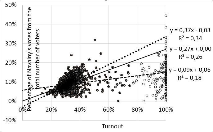
Figure 1. The results of the S-S method at different turnout discard thresholds for precinct election commissions
Modified method of Sobyanin-Soukhovolsky
Hence we may draw the conclusion that it makes sense to consider not the coefficient S-S itself, but the dependence of the linear regression coefficient \(a_j(\tau)\) on the turnout discard threshold \(\tau\) (that is, the value of the linear coefficient S-S calculated for the PEC, for which the turnout does not exceed the value of \(\tau\)). Figure 2 shows this dependence for the two main candidates for the Moscow mayoral election of 2013.
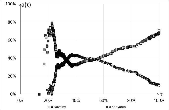
Figure 2. Dependence of the coefficient S-S on the turnout discard threshold
The traditional S-S method presupposes that the linear coefficient S-S is compared with the vote share received by the winner, calculated from the number of voters who took part in the elections \(v_j\). This indicator can also be shown on the graph, depending on the turnout discard threshold. The same can be done with a free coefficient S-S \(b_j\). Figure 3 shows three indicators depending on the turnout discard threshold \(\tau\) for the candidate Sobyanin S.S. (not to be confused with one of the authors of the method!) in the mayoral election in Moscow in 2013, and in Figure 4 there are the indicators of both Sobyanin and Navalny.
Figure 4 allows us to draw the following conclusions:
1) The traditional S-S method indicates the signs of fraud (since the linear coefficient S-S at 100% turnout is greater than the vote share received by Sobyanin, and the free S-S coefficient at 100% turnout is less than zero), but if we take into account only the precincts with a turnout up to 55%, this method indicates signs of fraud in favor of Navalny.
This fact shows that the traditional S-S method should be used with great caution.
2) Approximately to 37% turnout the vote share for Navalny kept increasing, and then it stabilized. Coefficients S-S demonstrate this effect more clearly than the exponent \(v\), since they are more sensitive to the turnout threshold.
3) The curves for Sobyanin and Navalny are symmetric. This is due to the fact that the remaining candidates did not compete with these two candidates. Votes were mainly shared between Sobyanin and Navalny. Voting for other candidates, as well as the presence of invalid ballots, will violate the symmetry of these curves.
4) At any turnout threshold, candidate Sobyanin is ahead of candidate Navalny by the vote share. However, there exists such a range of the turnout spectrum in which the linear coefficient S-S of Navalny is greater than the linear coefficient S-S of Sobyanin and the free coefficient S-S of Navalny is less than zero. In this area, the increase in turnout gave more advantages to Navalny than to his opponent.
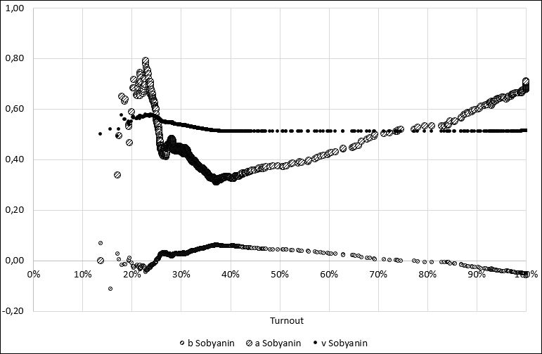
Figure 3. Dependence of electoral indicators of candidate Sobyanin from turnout
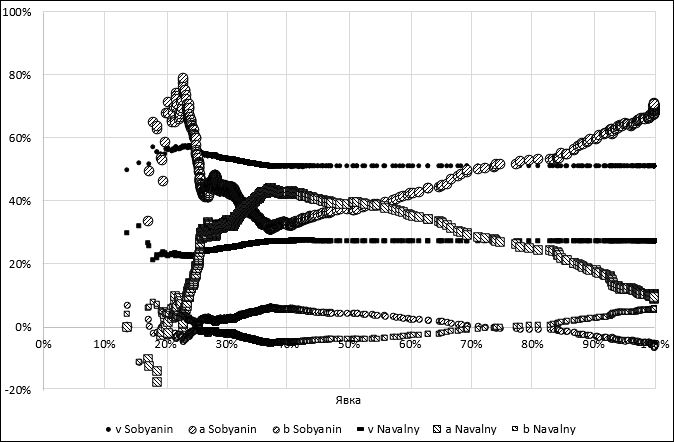
Figure 4. Dependence of electoral indicators of candidates Sobyanin and Navalny from turnout
Simulation experiments
To illustrate the behavior of the indicators \(v\), \(a\) and \(b\), a series of simulation experiments was carried out. The list of electoral commissions (PECs) and their amount (3374) were taken directly from the official statistics on the Moscow mayoral election of 2013.
The electoral behavior was simulated in the following way: each voter took a decision to participate in the elections with a probability \(q_i\) depending on number \(i\) of the precinct to which the voter was assigned. The voter who decided on voting had to choose from three options: with probability \(p_0\) he voted with an invalid ballot (which also simulated voting for all other candidates except the first and the second), with probability \(p_{i1}\) (depending on the number of the PEC to which the voter is assigned), he voted for the first candidate (or electoral association), and with probability \(1 - p_0 - p_{i1}\) he voted for the second candidate.
The probability \(p_0\) of invalid voting was assumed to be 5% in all experiments.
Experiments differed in the dependence of probabilities \(q_i\) and \(p_{i1}\) on \(i\), simulating electoral differences between polling stations (territories). In particular, these dependences could describe the statistical dependence of the values \(q_i\) and \(p_{i1}\).
Some experiments simulated electoral fraud either in the form of a random amount of ballot stuffing in some commissions, or in the form of ballot switching (that is, transferring a part of the votes cast for the second candidate to the first candidate) of a random amount of votes in some commissions.
Experiment 1. Quasi-homogeneous fair competitive elections
In this experiment, a society was simulated, in which the value \(q_i\) is a normal random variable with the given mathematical expectation \(M\) and a standard deviation \(\Sigma\) (we naturally replace \(q_i\) with zero or 100% if this random variable turned out to be less than zero or more than 1, respectively). The probability \(p_{i1}\) of voting for the first candidate is also a normal random variable with the given mathematical expectation \(m\) and standard deviation \(\sigma\). Thus, in this experiment we simulate a more or less homogeneous (quasi-homogeneous) community in which the turnout and vote shares are independent random variables.
(The community would have turned out even more homogeneous if \(q_i\) and \(p_{i1}\) did not depend on \(i\) at all – see experiment 3; the quasi-homogeneous community seems to be more realistic).
Figure 5 shows the behavior of the studied indicators in one of the experiments with \(M\)=40%, \(\Sigma\)=20%, \(m\)=60%, and \(\sigma\)=40% (this means that the average probability of voting for the second applicant equals 35%). It is easy to notice that in this case the linear coefficient S-S \(а\) coincides with exponent \(v\) with the high turnout discard threshold, and the free coefficient \(b\) is close to zero. At the same time, the winner’s share does not equal 60%. It is important that the candidates’ linear coefficients S-S vary considerably in the areas of average turnout and sometimes they even overlap. This indicates a high level of competition.
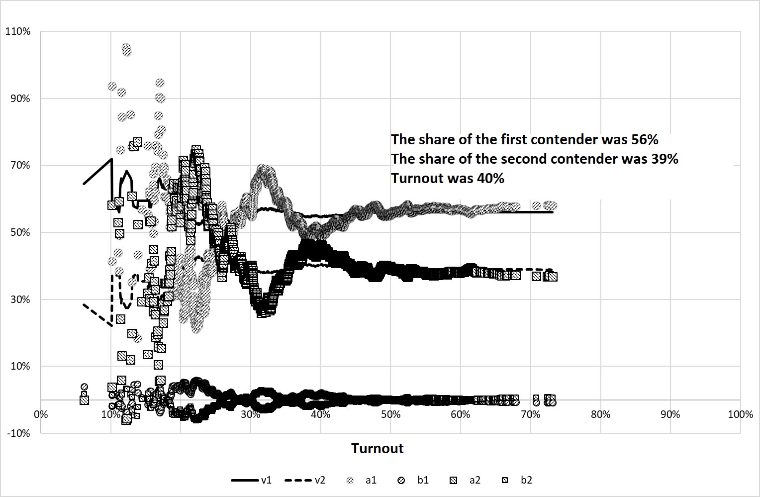
Figure 5. The results of Experiment 1
However, it should be noted that an increase in the level of turnout homogeneity (i.e., a decrease in the value of \(\Sigma\)) can lead to a deviation of the coefficients S-S from the balanced values.
Experiment 2. Heterogeneous fair competitive elections
If there is a statistical relationship between the turnout and vote share (and this relationship can be explained by different reasons), the coefficients S-S undergo deviations from the balanced values.
We will divide the election commissions into two unequal groups: the first includes 95% of the PECs, and the second – only 5%. In the first group, the value \(q_i\) is a normally distributed random variable with \(M\)=40%, \(\Sigma\)=10%, and the average voting for the first candidate is a normal random variable with \(m\)=47.5% and \(\sigma\)=40% (i.e., in this group the average vote share for the first and second candidates is the same).
In the second group, the value \(q_i\) is a normally distributed random variable with \(M\)=80%, \(\Sigma\)=10%, and the average vote share for the first candidate is a normal random variable with \(m\)=80% and \(\sigma\)=40%. Thus, the turnout and vote share are statistically dependent values.
Change of indicators in one of such experiments is shown in Figure 6.
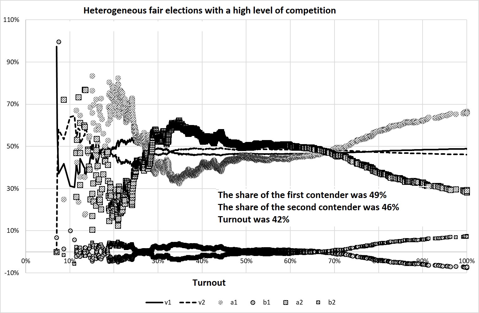
Figure 6. The results of Experiment 2
It can be seen that only 5% of PECs with specific electoral traditions make the coefficients S-S deviate greatly from the balanced values.
Experiment 3. Homogeneous and quasi-homogeneous elections with ballot stuffing
Figure 7 shows the result of the experiment with the ballot stuffing for the first candidate. The stuffing that takes place in half of the PEC consists in adding to the ballots actually received by the voters a certain number (in our case – a random number from 0 to 399) of ballots voting for the first candidate.
In this experiment, we deliberately made the turnout more homogeneous, i.e. assumed that \(\Sigma\)=0 for \(М\)=40%. This made it possible to make the effects of deviation of \(а\) from \(v\), and \(b\) from zero more vivid. Voting for the first and second candidate was on average equally probable (\(m\)=47.5%, \(\sigma\)=40%).
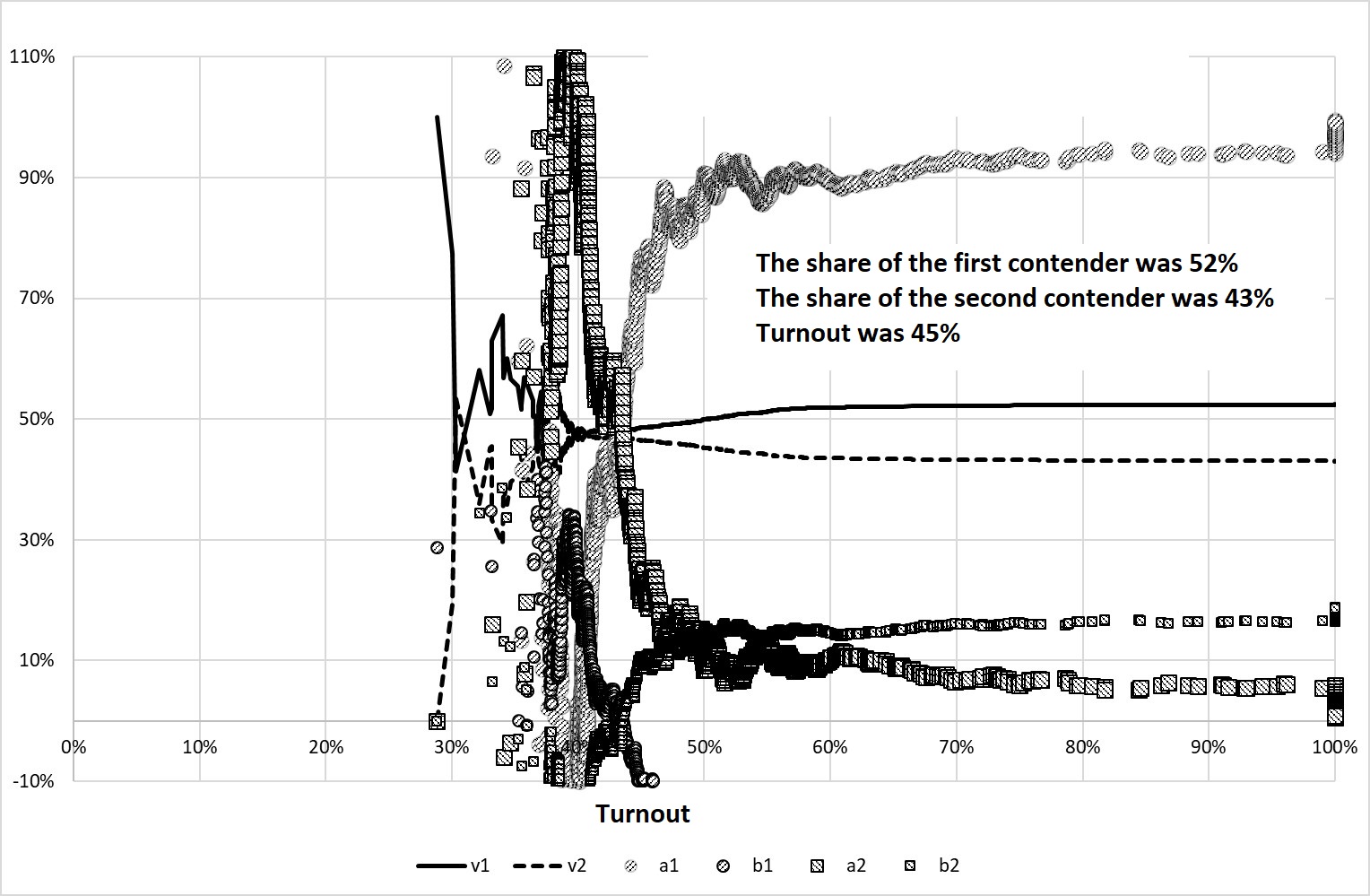
Figure 7. The result of Experiment 3
However, if the turnout is not as homogeneous as in the previous experiment, for example, if we assume that \(\Sigma\)=40% at \(М\)=40%, then the behavior of the coefficients S-S does not show the effect of the ballot stuffing – see Figure 8.
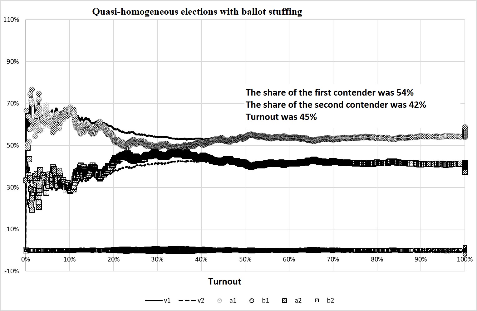
Figure 8. The result of Experiment 3
Experiment 4. Homogeneous competitive elections with ballot shifting
Figure 9 shows the behavior of the studied indicators in the experiment with \(M\)=40%, \(\Sigma\)=10%, \(m\)=47.5% and \(\sigma\)=40% (equally probable average voting for both candidates). In half of the election commissions, when counting votes a random number from 0 to 399 from the second candidate is taken away, and given to the first candidate (of course, it is taken into account that the number of votes should not be less than zero).
There is an interesting effect: the indicator \(а\) of the winner becomes less than the indicator \(v\), and the indicator \(b\) becomes more than zero. Thus, the traditional derivation of the S-S method is incorrect here, more precisely, the sign of fraud is the deviation of the coefficient \(а\) from \(v\) in the lower side, and the coefficient \(b\) in the positive region. This, by the way, means that by a skillful combination of ballot stuffing and ballot switching it is possible to achieve the effect when the coefficients S-S will take balanced values.
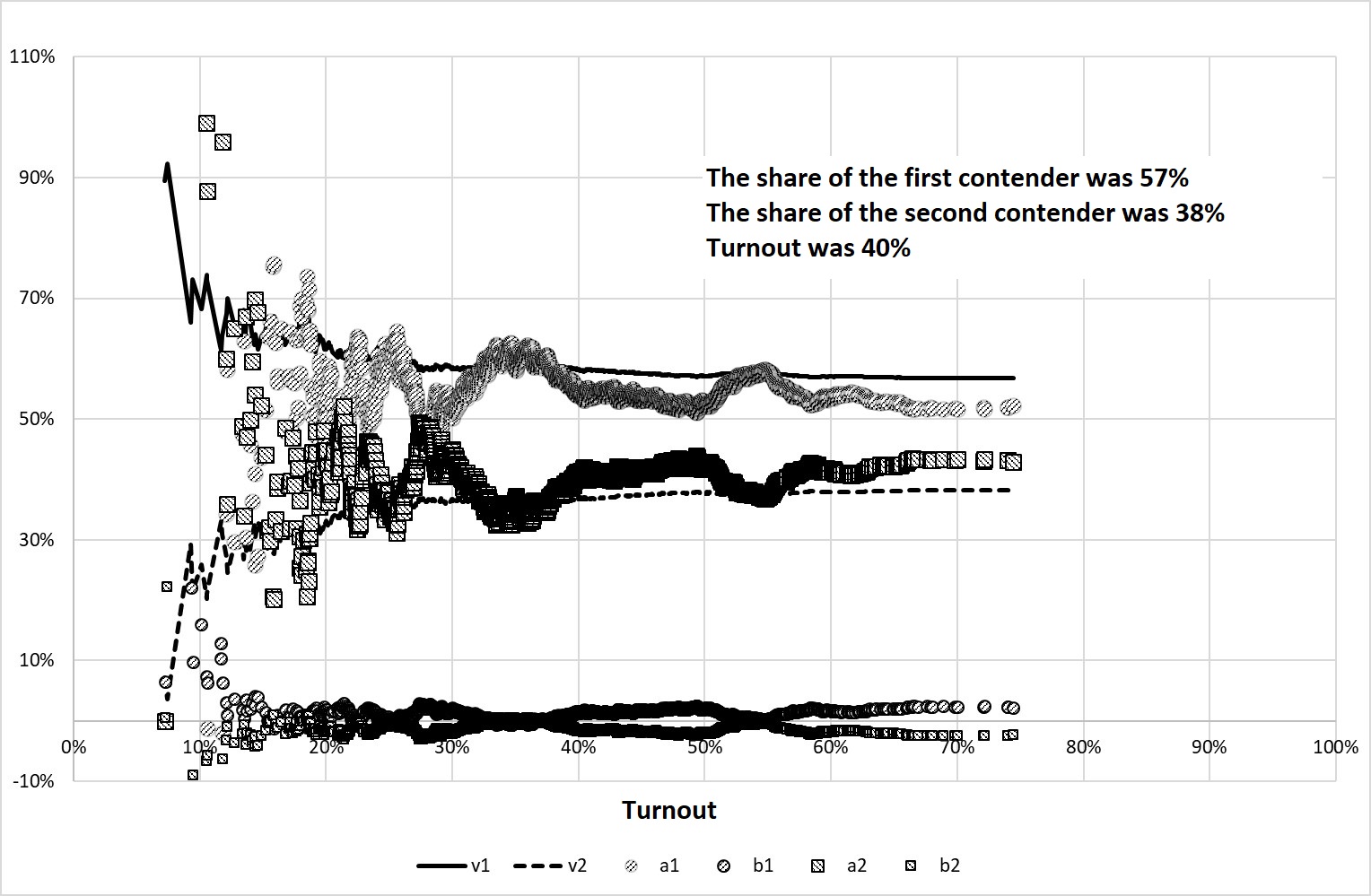
Figure 9. The result of Experiment 4
Conclusions
The traditional Sobyanin-Soukhovolsky method is poorly applicable to the search for signs of fraud for at least three reasons: firstly, it is very sensitive to statistical “emissions”; secondly, it can generate false signs of ballot-rigging; and thirdly, ballot-rigging, such as ballot switching can lead to wrong conclusions. However, in the modified form discussed in this article, Sobyanin-Soukhovolsky method is more useful: the character of the behavior of the three indicators – the two coefficients S-S and the average vote share of candidate \(v\), depending on the turnout discard threshold, can say more about the validity of voting and ballot counting.
Simulation experiments show that the characteristic behavior of the coefficients S-S has the form determined either by direct vote-rigging or by territorial heterogeneities in electoral behavior. Therefore, based on the behavior of these coefficients calculated on the basis of official electoral statistics, it is possible to make assumptions about the presence or absence of fraud, or about the existence of territorial differences in electoral behavior.
According to the behavior of these coefficients, it is also possible to evaluate in which area of the turnout value there are advantages to one or another candidate.
It should be noted that the real Russian electoral statistics gives expressive diverse examples of these indicators’ behavior.
Received 26.04.2018, revision received 14.06.2018.
References
- Buzin A.Yu., Lyubarev A.E. Prestuplenie bez nakazaniya: Administrativnye izbiratel’nye tekhnologii federal’nykh vyborov 2007–2008 godov [Crime without Punishment: administrative electoral technologies in federal elections 2007–2008]. Moscow: TsPK “Nikkolo M”; Tsentr “Panorama”. 2008. 284 p. (In Russ.)
- Buzin A.Yu. Vliyanie territorial'nykh neodnorodnostei i fal'sifikatsii na elektoral'nye pokazateli [Impact of Territorial Heterogeneity and Falsifications on Electoral Indicators]. - Vestik RUDN, ser.: matematika, informatika, fizika. 2014. No. 2. P. 72-80. (In Russ.)
- Kunov A., Myagkov M., Sitnikov A., Shakin D. Rossiya i Ukraina: neregulyarnye rezul'taty regulyarnykh vyborov, Analiticheskii doklad Instituta otkrytoi ekonomiki [Russia and Ukraine: irregular results of regular elections, Analytical Report of the Institute of Open Economy]. Мoscow.: 2005. 37 p. (In Russ.)
- Myagkov M., Ordeshook P.C., Shakin D. The Forensics of Election Fraud: Russia and Ukraine. New York: Cambridge University Press. 2009. 289 p.
- Sobyanin А.А., Sukhovolsky V.G., Demokratiya, ogranichennaya fal'sifikatsiyami: Vybory i referendumy v Rossii v 1991-1993 gg. [Democracy limited by fraud: Elections and referendums in Russia in 1991-1993]. Moscow.: Project Group on Human Rights.1995. 268 p. (in Russ.).